Chapter 6 Thermodynamic Properties of Fluids

งานนำเสนอเรื่อง: "Chapter 6 Thermodynamic Properties of Fluids"— ใบสำเนางานนำเสนอ:

1 Chapter 6 Thermodynamic Properties of Fluids
Measured properties: P, V, T, composition Fundamental properties: U (from conservation of energy) S (from directional of nature) Derived thermodynamics properties: Enthalpy: H = U + PV Helmholz energy: A = U – TS Gibbs energy: G = H – TS ในบทที่ 3 เราได้เรียนเรื่องสมบัติที่วัดได้คือ PVT และความสัมพันธ์ระหว่างสมบัติที่วัดได้ ตลอดจนเราทราบว่าสมัติที่บอก ไม่จำเป็นต้องบอกหมดทุกตัว บอกเพียงบางจำนวนเท่านั้น (Gibbs phase rule หรือ degree of freedom: a certain number of intensive properties of a system also fixes the values of all other intensive properties) บทนี้เราจะเรียน Thermodynamic property ก่อนอื่นเรามารู้จัก คำ ว่าสมบัติ มีสมบัติอะไรบ้าง Property:- measured, fundamental, and derived properties. สิ่งที่เราสนใจ เราไม่สนใจวัดสมบัติเฉพาะตัวใด ตัวหนึ่งเท่านั้น แต่สนใจวัดการเปลี่ยนแปลงสมบัติที่เราต้องการระหว่างสภาวะที่ 1 และ 2 หรือระหว่างกระบวนการ โดยเฉพาะอย่างยิ่ง  S, H เป็นต้น โดยใช้สมบัติที่วัดได้และเหมาะสมบางค่า จาก PVT จาก 1st และ 2nd law เราจะสร้าง fundamental property เราต้องการเชื่อม fundamental property และ thermodynamic property

2 Let’s consider the calculation of DU from state 1 to 2
Let’s consider the calculation of DU from state 1 to 2. The computational paths are assumed by picking the proper path. In considering paths, 2 things should be considered. (1) what property data are available? (2) what path yields the easiest calculation? Volume Temperature T1, V1 T2, V2 DUreal Step 1 Step 2 Step 3 การศึกษาวิชา Thermodynamics มีประโยชน์อย่างมาก ตัวอย่างเช่นการเปลี่ยนแปลงจากสภาวะที่ 1 ไป 2 จาก TV diagram นักศึกษาจะเห็นว่ากระบวนการจริงแสดงด้วยเส้นทึบ เราต้องการคำนวณค่า U แต่ไม่สามารถคำนวณได้โดยตรง เนื่องจากไม่มีความสัมพันธ์หรือสมการที่เราจะนำมาใช้ได้ สิ่งที่ทำได้คือการลองสมมุติวิถีการเปลี่ยนแปลงใหม่จากสภาวะที่ 1 ไป 2 และสามารถหาความสัมพัน์ทางคณิตศาสตร์มาใช้ได้ การเลือกวิถีเพื่อใช้ในการคำนวณจึงสำคัญ เลือกแล้วควรคำนวณง่าย Hypothetical path Real path

3 เราสามารถแสดงการเปลี่ยนแปลงของ F โดยใช้ Exact differential equation:
Thermodynamics property relationships: Independent and dependent property Exact differential equation เราได้เคยเห็นข้อความนี้มาแล้วในการเรียนบทที่ 3 ถ้าเรามีสมบัติที่เป็นอิสระกัน 2 ค่า สมบัติตัวที่ 3 จะเป็น dependent property เราสามารถแสดงการเปลี่ยนแปลงของ F โดยใช้ Exact differential equation: the integral of dF is independent of path. F/x จะขึ้นกับ วิถีการเปลี่ยนแปลง (path)

4 Any two variables may be chosen as the independent variables for the single component, one-phase system, and the remaining six variables are dependent variables. For example: U = U(T,V), U = U(T,P), U = U(T,S), U = U(H,S), We can use any of the forms of U with other two independent variables, but it turns out that the properties T and V are particularly convenient choices for U calculation.

5 The 1st law of Thermodynamics
Energy is conserved. System Q W + - Closed system: d(nU) = dQrev + dWrev Open system: d(nH) = dQrev + dWrev in these cases we negelect the change in PE and KE

6 The 2nd law of Thermodynamics
Entropy (S) is conserved only in internal reversible process. Entropy of the universe always increases. Know direction of the process. Qrev = Td(nS) Internal reversible process: S = 0 Real process (irreversible process): S > 0 Impossible process: S < 0

7 Thermodynamic Properties of Fluids
System Q W - + 1st Law d(nU) = dQ + dW d(nU) = dQrev + dWrev dWrev = - Pd(nV) 2nd Law dQrev = Td(nS) Combine 2 laws: d(nU) = Td(nS) – Pd(nV) สมการแรกเป็นสมการของ 1st law สมการที่ 2 แสดงให้กระบวนการที่ภายในเป็น reversible process แต่สิ่งแวดล้อมไม่จำเป็น เราแทนงานด้วย Pd(nV) work และแทน Q ด้วยกฎข้อที่ 2 จะเห็นว่าเราได้ค่าการเปลี่ยนแปลง U จาก 1st law และ 2nd law of thermodynamics. ข้อสังเกตคือเราได้สมการนี้มาจากกระบวนการที่เป็น internal reversible process แต่ค่าที่แสดงการเปลี่ยนแปลงเป็นสมบัติของระบบ แสดงว่าสมการนี้ใช้ในการคำนวณค่า U ของกระบวนการอื่น ๆ ได้ เพราะ สมบัติของระบบไม่ขึ้นกับวิถีการเปลี่ยนแปลง แต่ขึ้นกับสภาวะของระบบเท่านั้น แต่ต้องจำไว้ว่าสมการนี้ใช้สำหรับระบบปิดหรือระบบที่มีมวลคงที่เท่านั้น เมื่อพิจารณาสมการสุดท้าย จะเห็นว่า มีสมบัติ P V T U และ S

8 Thermodynamic Properties of Fluids
Enthalpy H = U + PV Helmholtz energy A = U – TS Gibbs energy G = H – TS เขียนในรูป Differentiation equation d(nH) = d(nU) + Pd(nV) + (nV)dP d(nA) = d(nU) – Td(nS) – (nS)dT d(nG) = d(nH) – Td(nS) – (nS)dT These equation are Fundamental property relations. คำถาม ทำไมต้องนิยามสมบัติพวกนี้ขึ้นมาอีก นิยาม H เพราะ 1st law ค่า S เพราะ 2nd law เราคงสงสัยว่า เรานิยามค่า A และ G ขึ้นมาเพื่ออะไร ตอนนี้อาจจะยังตอบคำถามนี้ไม่ได้ แต่ขอให้เราทราบว่าทั้ง G และ A เป็น State function เพราะเกิดจากการรวมกันของ state function

9 Free Energy A: Helmholtz energy A = U –TS dA = dU –TdS = Q + W – TdS
= TdS + Wrev – TdS A = Wrev the change in A is the maximum work output from the system. A is a new function that indicates the direction of the process at constant T and V. For a constant T process the Helmholtz free energy gives all the reversible work. For this reason the Helmholtz free energy is sometimes called the "work function."

10 If T and V are constant: W = 0 dU - Q  0 dU - TdS  0 dA  0
Closed system dU = Q + W dU - Q - W = 0 2nd law of TD: dU - Q - W  0 If T and V are constant: W = 0 dU - Q  0 dU - TdS  0 dA  0 AT,V  0 Spontaneous process tries to decrease A or keeps A minimum. We conclude that for a process at constant temperature and volume the Helmholtz free energy seeks a minimum. Any spontaneous process in a system at constant T and V must decrease the Helmholtz free energy (if the system is away from equilibrium) or leave the Helmholtz free energy unchanged (if the system is at equilibrium).

11 Free Energy G: Gibbs energy
G = H –TS Constant T; G = U + PV –TS = A + PV Constant P; dG = dA + PdV dA = dG –PdV Wnet = Wmax,rev - PdV Wnet = -dG + PdV - PdV Wnet = -dG For the process with T and P constant, G is the maximum work output that extracts from the process. Pext PdV

12 Most process is at constant T and P;
G = 0 equilibrium at constant T and P. G < 0 Spontaneous change at constant T and P. G is a new function that indicates the direction of the process at constant T and P. That is, at constant T and p the Gibbs free energy seeks a minimum. Any spontaneous process in a system at constant T and p must decrease the Gibbs free energy (if the system is away from equilibrium) or leave the Gibbs free energy unchanged (if the system is at equilibrium).

13 d(nA) = - Pd(nV) – (nS)dT d(nG) = (nV)dP – (nS)dT
จัดรูปสมการใหม่ d(nU) = Td(nS) – Pd(nV) d(nH) = Td(nS) + (nV)dP d(nA) = - Pd(nV) – (nS)dT d(nG) = (nV)dP – (nS)dT ทั้งหมดเป็น Exact Differential Equation These equations can be used in any process. We group properties together: U S V, H S P, A T V G T P

14 ถ้า n = 1 mol dU = TdS – PdV dH = TdS + VdP dA = - PdV – SdT
dG = VdP – SdT ถ้าใช้หลักของ exact differential equation กับทั้ง 4 สมการ จะได้ความสัมพันธ์ใหม่ที่เรียกว่า Maxwell’s equation These equations can be used in any process. We group properties together: U S V, H S P, A T V

15 All properties on the left hand side are measured PVT data
All properties on the left hand side are measured PVT data. So they enable us to calculate U, H and G. ให้นักศึกษาสังเกต Maxwell equation แล้วสรุป จะเห็นว่าด้านซ้ายของสมการเป็นสมบัติที่วัดได้ โดยเฉพาะอย่างยิ่ง เป็น PVT ส่วนสมการทางขวามือ เป็นสมบัติ thermodynamics ซึ่งวัดได้ Maxwell’s Equation

16 We group properties together: fundamental grouping (U, S, V) (H, S, P)
(A, T, V) (G, T, P) These equations can be used in any process. These properties are group exclusively with measured properties P V T.

17 Other useful mathematic relations
These equations can be used in any process. These properties are group exclusively with measured properties P V T.

18 These equations can be used in any process.
These properties are group exclusively with measured properties P V T. ค่า derivative ที่ใช้แทนกันได้คือ Maxwell relation Any derivatives presnted in this figure can be rewritten by following a path in the diagram to ultimately lead to Cv, Cp, B, K and EOS.

19 การหา DH และ DS ในรูปของ T และ P
จาก H = U + PV dH = dU + PdV + VdP จาก dU = TdS – PdV dH = TdS + VdP หารด้วย dT ตลอด และกำหนดให้ P คงที่ dU + PdV = TdS มาจากการรวม 1st และ 2nd law of thermodynamics

20 การหา DH ในรูปของ T และ P
จาก dH = TdS + VdP หารด้วย dP ตลอด และกำหนดให้ T คงที่ จาก H = H(T,P) และ S = S(T,P) และเป็น Exact Differential Equation

21 เรามักคำนวณค่า DH มากกว่าที่จะคำนวณค่า H
กิจกรรมกลุ่ม เกี่ยวกับการกำหนด Reference state เรามักคำนวณค่า DH มากกว่าที่จะคำนวณค่า H จึงมักกำหนด Reference state ให้มี H = 0 แล้วคำนวณ DH จากสมการข้างบนนี้แทน

22 การหา DS ในรูปของ T และ P
ในทำนองเดียวกัน เรามักคำนวณค่า DS มากกว่าที่จะคำนวณค่า S จึงมักกำหนด Reference state ให้มี S = 0 แล้วคำนวณ DS จากสมการข้างบนนี้แทน

23 การหา DU ในรูปของ T และ V
จาก dU = TdS – PdV หารด้วย dT แล้วกำหนดให้ V คงที่ และอีกสมการหารด้วย dV แล้วกำหนดให้ T คงที่ จากคุณสมบัติของ exact differential equation ของ U = U (T,V) และ S = S (T,V) และใช้ Maxwell’s equation ก็จะได้สมการข้างบน

24 The Ideal Gas State

25 For H & S and  U &  S calculations, we use the relationships of heat capacity of substances and temperature. Students are advised to review the physical meaning of heat capacity in both constant pressure or volume processes and of ideal gas. นศ. ควรศึกษาตัวอย่างที่ 6.1 ในหน้า 204 ซึ่งเป็นการคำนวณ DH และ DS ของการเปลี่ยนแปลงของน้ำของเหลวจาก 1 bar 25C ไปเป็น 1000 bar 50C โดยโจทย์กำหนดค่า Cp, V และ  มาให้ แต่เนื่องจากทุกค่าเป็นค่าที่ T และ P ต่าง ๆ ดังนั้นจึงใช้การคำนวณทางอ้อมแทน ดังนี้ 1 bar 25C  bar 50C  bar 50C Isobaric process Isothermal process นศ. อาจใช้ข้อมูลจาก Steam Table มาเปรียบเทียบการคำนวณก็ได้

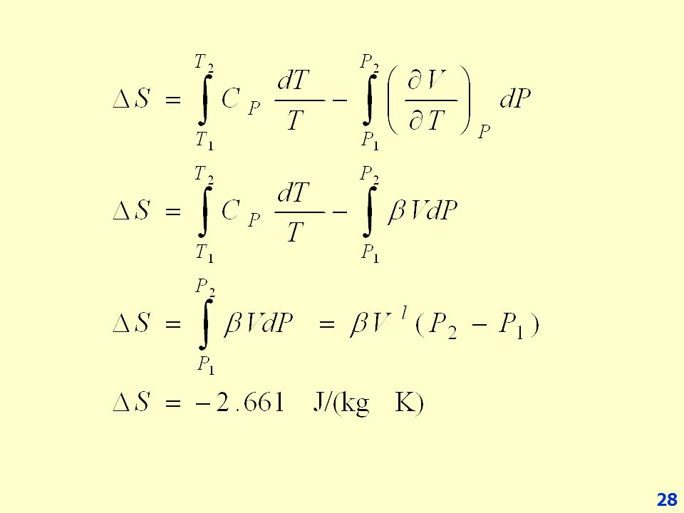
26 Example 1 (problem 6.7) Estimate the change in enthalpy and entropy when liquid ammonia at 270 K is compressed from its saturation pressure of 381 kPa to 1200 kPa. For saturated liquid ammonia at 270 K, Vl = 1.551x10-3 m3 kg-1 and b = 2.095x10-3 K-1

27

28

29 Homework # Problem # 6.9

30 The Gibbs Free Energy จาก dG = VdP – SdT 6.10 G = G(P,T)
เราได้ derive สมการที่ 6.10 มาแล้ว จะเห็นว่าเ G เป็น function ของ T และ P หรือเราอาจพูดได้ว่าสำหรับสารบริสุทธิ์ เฟสเดียวแล้ว เราสามารถแสดงค่าของแต่ละ thermodynamic property U H A G เป็น function ของสมบัติ 2 ค่าได้ ถ้าเรานำค่า G มาหารด้วย RT แล้ว Diff G/RT จะได้สมการในบรรทัดทัดที่ 3 จากนั้นแทนค่า G จากสมการที่ 6.10 ในค่า dG และแทนค่า G = H-TS ในค่า G ที่เทอมที่ 2 ของสมการ ข้อสังเกตคือ ทุกเทอมในสมการ เป็นเทอมไร้หน่วย และค่า G อยู่ในรูปของ V และ H ไม่ใช่ P และ S เหมือนสมการที่ 6.10 6.37

31 จัดรูปสมการใหม่ 6.38 6.39 แสดงว่า G/RT เป็นฟังก์ชั่นของ P, T, V/RT และ H/RT และจาก G = H – TS และ H = U + PV จากสมการที่ 6.37 เราจัดเทอมใหม่ นศ. จะเห็นว่าเราหาค่าสมบัติตัวอื่น ๆ ได้ในรูปของ G/RT ดังแสดงในสมการที่ แสดงว่า G/RT หรือ G เป็นฟังก์ชั่นของ P, T เราเขียนได้ในรูป G/RT = g(T,P) เราสามารถหาค่า thermodynamic property ได้ในรูปของสมการง่าย ๆ

32 นศ. เห็นความสำคัญของค่า G หรือไม่. …
นศ. เห็นความสำคัญของค่า G หรือไม่ ?? …..G เป็นตัวกำหนดหรือเป็นตัวเชื่อมกับค่าสมบัติทางเทอร์โมไดนามิกส์ตัวอื่นๆ ที่สมบูรณ์ที่สุด G จึงเป็น Generating function แม้ว่า G จะมีความสำคัญก็ตามในแง่ของความสัมพันธ์กับสมบัติตัวอื่น ๆ แต่การหาค่า G ทำได้ยากมาก ยังไม่ทราบว่าจะทำการทดลองอย่างไร ปัญหาอยู่ที่ว่าทำอย่างไรจึงจะทำงานต่อได้

33 Residual Property Residual Gibbs Energy GR = G – Gig เป็นสมบัติที่ก๊าซจริงเบี่ยงเบนจาก Ideal gas ที่สภาวะที่มี T และ P เท่ากัน ถ้า M เป็นสมบัติใด ๆ MR = M – Mig จึงมีการนิยามเทอมใหม่ขึ้นมาอีก ขอให้นักศึกษาสังเกตว่า มีการหาทางแก้ปัญหาหรือหาทางออกเสมอเมื่อมีปัญหา มีการกำหนดเทอมใหม่ขึ้นมาเพื่อเป็นตัวเชื่อมกับสภาวะที่เป็นอุดมคติ หรือเบี่ยงเบนออกจากสภาพที่เป็นอุดมคติ ตัวนี้เป็นตัวที่ 2 ถ้านับค่า Z เป็นตัวที่ 1 สมบัติตัวอื่น ๆ สามารถเขียนให้อยู่ในรูป residual property ได้ เช่นเดียวกัน

34 เช่น VR = V – Vig

35 จาก GR = G – Gig จากสมการที่ 6.37 เราสามารถเขียนในรูปของ G และ Gig ได้

36 ในทำนองเดียวกับสมการที่ 6.38
ในทำนองเดียวกัน และจากสมการของ V/RT, H/RT, S, U เราสามารถเขียนให้อยู่ในรูปของทั้งก๊าซจริงและอุดมคติ ในที่นี้แสดงให้เห็นเฉพาะ residual property

37 ในกรณีที่ T คงที่ การใช้สมการที่ 47 และ 48 ทำได้โดยหาค่า Z และ (Z/T) จาก PVT data ที่ได้จากการทดลอง จากนั้นหาค่า integrand จากการทำ integration หรือทำ graphical method ถ้าเรามี EOS ของ PVT ในรูป Z เราสามารถหาค่า HR และ SR ได้ หาค่า GR ได้โดยการ plot (Z-1)/P กับ P หาค่า HR ได้โดยการ plot (Z/T)P/P กับ P หาค่า SR ได้โดยการ plot (Z-1)/P กับ P

38 มักกำหนด Reference state ที่ P0 T0 ในการคำนวณค่า Hig และ Sig
นศ. จะเห็นว่าสมการของ ideal gas มีประโยชน์ในการคำนวณค่า HR และ SR หรือ Residual property เป็นค่าที่ใช้ได้ดีในการคำนวณค่า H ของทั้งของเหลวและก๊าซ กรณีที่เป็นก๊าซนั้นค่า HR และ SR จะมีค่าน้อยมาก ส่วนค่า HR และ SR ของของเหลวนั้นมีค่าสูงกว่าเนื่องจากมีการรวมค่า H และ S ของการระเหยเข้ามาด้วย ในการคำนวณนั้น เราเน้นที่ H และ S จะสะดวกมาก ถ้าเราสภาวะมาตรฐาน การเลือกสภาวะมาตรฐาน P0 และ T0 นั้นขึ้นอยู่กับความสะดวกในการคำนวณ และค่าตัวเลขที่จะให้ต่อ และ เดิมเราเคยคิดกันว่า Ideal gas equation นั้นไม่ดี แต่ตอนนี้เราพบว่าสมการของ Ideal gas และ heat capacity ของ ideal gas นั้น ช่วยเราในการคำนวณเป็นอย่างมาก

39 การบ้าน ให้นักศึกษาอ่านเรื่อง Residual properties in the Zero-pressure limit หน้า 210 แล้ว เขียนสรุปความยามไม่เกินหนึ่งหน้ากระดาษ A4 ส่งทาง ในวันพุธที่ 27 มค. 2553 ที่

40 คำนวณค่า H และ S อธิบายสมการแต่ละเทอม

41 คำนวณค่า H และ S แสดงว่าเราได้สมการการหาค่าการเปลี่ยนแปลง H และ S ของก๊าซจริง ได้ในรูปของ residual property ปัญหาต่อไปที่เราจะต้องคิดคือเราจะหาค่า residual property ได้อย่างไร

42 HR and SR calculation 1. From experimental PVT data HR - Calculate Z plot Z vs any P determine (Z/ T)P calculate (Z/ T)P/P plot (Z/ T)P/P vs P

43 From experimental PVT data SR - Calculate (Z-1)/P - plot (Z-1)/P vs P

44 2. From the Virial EOS

45 3. From an appropriate EOS use the basic principles from chapter 3 to calculate the value of Z and (Z/ T)P q and I depends on each EOS

46 Case I:   

47 Case II:  = 

48 4. From generalized correlation
Z = Z0 + Z1 ซึ่งเราสามารถเริ่มต้นจากการทราบค่า Pr และ Tr แล้วเปิด Lee/Kesler Generalized-correlation Tables ในAppendix E

49 4. From generalized correlation (cont.) - the 2nd Vrial coefficient
เราสามารถหาค่า Residual property ได้จากการใช้ 2nd virial coefficient ได้ ซึ่งรูปแบบของสมการก็จะคล้ายกับค่า Z คือมีค่าที่ 0 และ1

50 the 2nd Virial coefficient

51 However, we are interested in DH and DS

52 Example 2 Calculate Z, HR and SR by the Redlich/Kwong equation for acetylene at 300 K and 40 bar and compare the result with value found from suitable generalized correlation and the 2nd virial coefficient. (Problem # 6.14)

53 Properties of acetylene: Tc = 308. 3 K Pc = 61. 39 bar w = 0
Properties of acetylene: Tc = K Pc = bar w = Tr = 300 K/308.3 K = Pr = 40 bar/61.39 bar =

54

55 Solution

56 Find the value of I, Case I:   
Substitute all values in Eq and 6.77, then you can find the value of HR and SR

57 the 2nd Virial coefficient

58 - the 2nd Vrial coefficient
เราสามารถหาค่า Residual property ได้จากการใช้ 2nd virial coefficient ได้ ซึ่งรูปแบบของสมการก็จะคล้ายกับค่า Z คือมีค่าที่ 0 และ1

59 Lee/Kesler generalized correlation

60 Two-phase system in equilibrium
สมการนี้แสดงให้เห็นถึงความสัมพันธระหว่าง latent heat of vaporization และ Psat เราเรียกสมการนี้ว่า Clausius-Claperon equation ยังมีสมการอีกสมการหนึ่งที่แสดงความสัมพันธ์ Temperature dependence of the vapor pressure of liquid หรือที่ นศ. รู้จักในสมการ Antoin Equation ln Psat = A – B/(T+C)

61 For Gas Mixture

62 Homework 6.44, 6.49, 6.51, 6.58, 6.88 (a)

63 การบ้าน ให้ศึกษาตัวอย่างทุกตัวอย่างในตำรา รวมทั้งการบ้านทุกข้อ ตั้งแต่บทที่ 3 และ 6 ในชั่วโมงติว จะจับฉลากหากลุ่มที่โชคดี แล้วให้แบ่งกลุ่มมาอธิบาย กลุ่มละ 3 คน ให้แบ่งกลุ่มเอง