2.3.2 Contrast Stretching Contrast

งานนำเสนอเรื่อง: "2.3.2 Contrast Stretching Contrast"— ใบสำเนางานนำเสนอ:

1 2.3.2 Contrast Stretching Contrast
The contrast of an image is its distribution of light and dark pixels Fig Low and high contrast histogram.

2 Contrast Stretching Contrast stretching Clipping thresholding

3 Contrast Stretching, a = 80, b= 160

4 Basic Contrast Stretching
Original Image Basic Contrast Stretching End-in Search

5 Original Image Convert Image Contrast Stretching

6 Red Green Blue

7 /********************************************
* Func: auto_contrast_stretch * Desc: performs basic contrast stretching on an image * Params: source - pointer to source image * cols - number of columns in the image * rows - height of image * ********************************************* void auto_contrast_stretch(image_ptr source, int cols, int rows) { long i; /* loop variable */ long number_of_pixels; /* total number of pixels in image */

8 long histogram[256]; /* image histogram */
unsigned char LUT[256]; /* Look-up table for point process */ int lowthresh, highthresh; /* lower and upper thresholds */ float scale_factor; /* scaling factor for contrast stretch */ /* compute histogram */ number_of_pixels = (long)cols * rows; for(i=0; i<256; i++) histogram[i]=0; for(i=0; i<number_of_pixels; i++) histogram[source[i]]++;

9 /* compute low and high thresholds */
for(i=0; i<256; i++) if(histogram[i]) { lowthresh = i; break; } for(i=255; i>0; i--) highthresh = i;

10 printf("Low threshold is %d High threshold is %d\n",
lowthresh,highthresh); /* compute new LUT */ for(i=0; i<lowthresh; i++) LUT[i]=0; for(i=255; i>highthresh; i--) LUT[i]=255;

11 scale_factor = 255.0 / (highthresh-lowthresh);
for(i=lowthresh; i<=highthresh; i++) LUT[i]=(unsigned char)((i - lowthresh) * scale_factor); /* transfer new image */ for(i=0; i<number_of_pixels; i++) source[i] = LUT[source[i]]; }

12 2.3.3 Intensity transformations
Digital negative Applications Display of medical images Produce negative prints of images Intensity level slicing Applications : Segmentation of certain gray level regions

13 Intensity transformations
Convert an old pixel into a new pixel based on some predefined function Implemented with simple look-up tables Simple transformation Null transform new pixel = old pixel Image negative y = -x+255 Gamma correction function Brightness of an image can be adjusted with a gamma correction transformation

14 Intensity transformations
Posterizing reduces the number of gray levels in an images Thresholding results when number of gray levels is reduced to 2. A bounced threshold reduces the thresholding to a limited range and treats the other input pixels as null transformation Figure 2.18(pp.63) Fig (a) 8-Level posterize transformation; (b) posterized image; (c) threshold transformation; (d) threshold image; (e) bounded threshold; (f) bounded threshold image.

15 Intensity transformations
Gamma correction Original gamma=0.45 gamma=2.20

16 Intensity Transformation
Intensity transformation is a point process that converts an old pixel into a new pixel base on some predefined function. This transformation is implemented with the LUT with ease. Gamma Correction

17 Intensity Transformation

18 Intensity Transformation

19 Intensity Transformation

20 Intensity transformations
Fig (a) Gamma collection transformation with gamma=0.45; (b) gamma collected image; (c) gamma collection transformation with gamma=2.2; (d) gamma collected image. Fig (a) Null transformation; (b) image; (c) negative transformation; (d) negative image. Page 60. 참조

21 Intensity transformations
Fig (a) Contrast stretch transformation; (b) contrast stretched image; (c) Contrast compression transformation; (d) contrast compressed image. Fig (a) 8-Level posterize transformation; (b) posterized image; (c) threshold transformation; (d) threshold image; (e) bounded threshold; (f) bounded threshold image. Page 62. 참조

22 Intensity transformations
Fig (a) 2-bit bit-clipping transformation; (b) resulting image. Fig (a) Iso-intensity contouring transformation; (b) contoured image. Fig Bit clipped image contrast stretched. Page 64. 참조

23 Intensity tranformations
Fig (a) Range-highlighting transformation; (b) resulting image. Fig (a) Solarize transformation using a threshold of 150; (b) solarize image. Page 65. 참조

24 Fig (a) First parabola transformation; (b) transformed image; (c) second parabola transformation; (d) second transformed image.

25 HW – 03 a) Plot กราฟ histogram

26 HW – 03 b)

27 สจพ 2.4 Frequency-based Operations Fourier Transform MTCT DI&SP

28 Spatial Frequency Efficient data representation
Provides a means for modeling and removing noise Physical processes are often best described in “frequency domain” Provides a powerful means of image analysis

29 What is spatial frequency?
Instead of describing a function (i.e., a shape) by a series of positions It is described by a series of cosines Fourier series Fourier Transform

30 สจพ 1-D Fourier Transform MTCT DI&SP

31 Our starting place is the observation that a periodic function may be written as the sum of sines and cosines of varying amplitudes and frequencies.

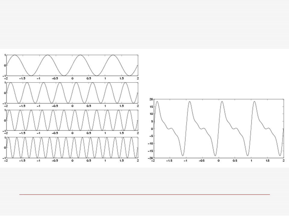
32 it is possible to form any function as a summation of a series of sine and cosine terms of increasing frequency For example, in figure we plot a function, and its decomposition into sine functions.

33 f(t)

34 We take the first three terms only (blue, green, red) to provide the approximation of the original function (purple). The more terms of the series we take, the closer the sum will approach the original function.

35 (1) where (2) Original function (purple) sines and cosines
Fourier coefficient Equations 1 and 2 are called Fourier transform pairs, and they exist if f(t) is continuous and integrable, and F(k) is integrable. These conditions are usually satisfied in practice.

36 f(t) => time-domain
1 2 3 4 1 F(u) => frequency-domain 3 II 4 2

37 Any function can be represented in 2 formats:
1) time-domain representation, f(t), or spatial domain, f(x), and 2) frequency-domain representationor Fourier domain, F(u) In other words, any space or time varying data can be transformed into a different domain called the frequency space.

38 Time-domain Frequency-domain

39 FT properties: If F(u) and G(u) are FT of function f(t) and g(t), respectively, Time scaling Frequency scaling

40 Time shifting Frequency shifting

41 Convolution theorem Correlation theorem

42 สจพ 2-D Fourier Transform MTCT DI&SP

43 แนวความคิดของการแปลงฟูเรียร์สามารถนำมาใช้กับฟังก์ชั่นหรือสัญญาณ 2 มิติ เช่น ภาพ ซึ่งจะเป็นการแปลงฟังก์ชั่นบน spatial domain (รูปภาพ) ไปเป็น frequency domain สมการคณิตศาสตร์แสดงความสัมพันธ์นี้เป็นดังนี้ IFT FT

44 ภาพแสดงความสัมพันธ์ระหว่างภาพใน spatial domain และความถี่ใน frequency (or Fourier) domain

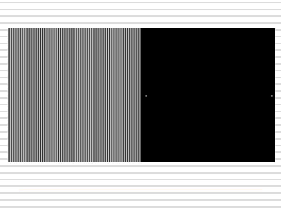
45 พบว่าระยะถี่-ห่างทางตำแหน่งในภาพ (x-y ใน spatial domain) จะแปลงไปเป็นจุดใน frequency domain (u-v)
โดยบริเวณที่มีระยะห่าง (ซึ่งมีความถี่ทางตำแหน่งต่ำ) เช่น บริเวณตัวบ้านรวมทั้งหน้าต่าง-ประตู จะไปอยู่ในตำแหน่งที่ใกล้จุดกำเนิด และในทางกลับกันบริเวณที่มีระยะถี่ (ซึ่งมีความถี่ทางตำแหน่งสูง) เช่น บริเวณที่มีลวดลายบนหลังคาบ้าน จะไปอยู่ในตำแหน่งที่ไกลจุดกำเนิดออกไป

46

47

48

49

50

51

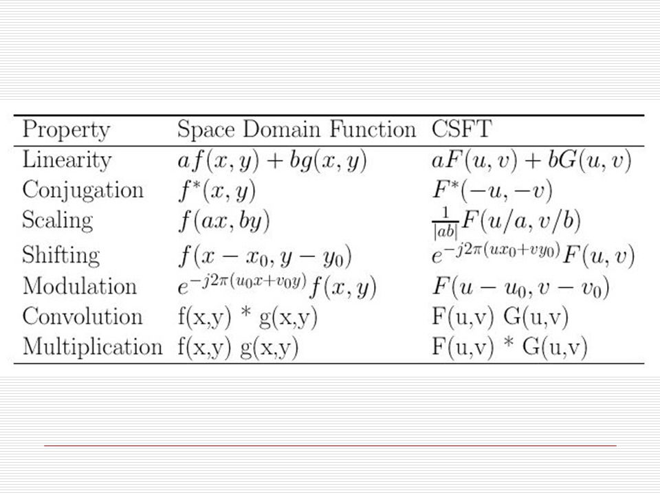
52 คุณสมบัติของการแปลงแบบฟูเรียร์ 2 มิติ (Properties of the 2-D Fourier Transform)

53

54 การแปลงแบบฟาส์ทฟูเรียร์ (The Fast Fourier Transform)
ในกรณีที่ข้อมูลเป็นปริมาณเต็มหน่วย (discrete) ดังเช่นภาพที่ถูกนำเข้าสู่ระบบคอมพิวเตอร์ การแปลงฟูเรียร์ข้างต้นยังคงใช้ได้อย่างสะดวกหลังจากมีการปรับปรุงแล้ว โดยสมการคณิตศาสตร์ของความสัมพันธ์คู่นี้จึงเป็นแบบเต็มหน่วย (Discrete Fourier Transform-DFT) เป็นดังนี้

55 สำหรับภาพที่มีขนาด NxM จะได้

56 เมื่อต้องการใช้คอมพิวเตอร์ประมวลผลการแปลงนี้ จำเป็นต้องใช้ขั้นตอนวิธี (algorith-m) ที่รวดเร็วและมีประสิทธิภาพ ดังนั้นจึงมีผู้เสนอขั้นตอนวิธีที่เรียกว่า (The Fast Fourier Transform-FFT) และได้รับความนิยมอย่างกว้างขวาง

57 Spatial Frequency or How I learned to love the Fourier Transform
Jean Baptiste Joseph Fourier

58 2.5 Group-based Operations Convolution Operation
สจพ 2.5 Group-based Operations Convolution Operation MTCT DI&SP

59 แล้วเลื่อน kernel นี้เพื่อไปหาค่าใหม่ของจุดภาพถัดไป
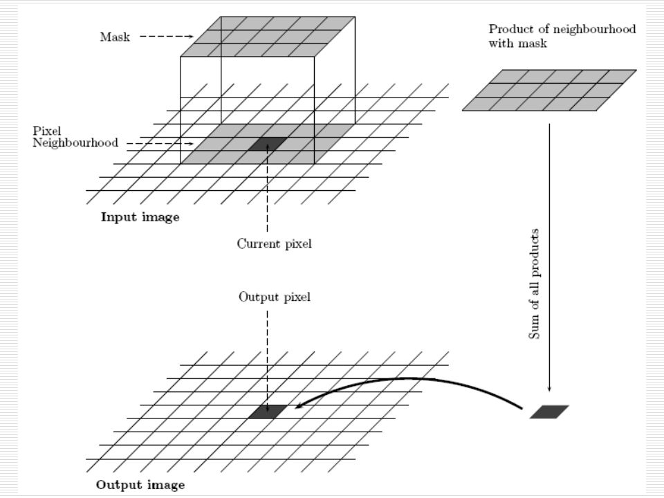
สจพ การกระทำแบบคอนโวลูชั่นเป็นการหาค่าใหม่ของจุดภาพใด ๆ โดยพิจารณาระบบเพื่อนบ้าน (Neighbors System) ในขั้นแรกจะต้องกำหนด window หรือ kernel ซึ่งเป็นตารางสี่เหลี่ยมจตุรัสขนาด 3x3, 5x5 หรือขนาดอื่น ๆ แต่ละช่องของตารางนี้จะถูกกำหนดให้มีค่าน้ำหนัก (Weights) โดยแต่ละช่องอาจมีค่าเท่ากันหรือไม่ก็ได้ จากนั้นนำ kernel นี้มาทาบบนภาพและหาบวกของผลคูณระหว่างค่าน้ำหนักกับค่าความเข้มบนจุดภาพ แล้วเลื่อน kernel นี้เพื่อไปหาค่าใหม่ของจุดภาพถัดไป MTCT DI&SP

60

61