ดาวน์โหลดงานนำเสนอ
1
Mathematical Model of Physical Systems

2
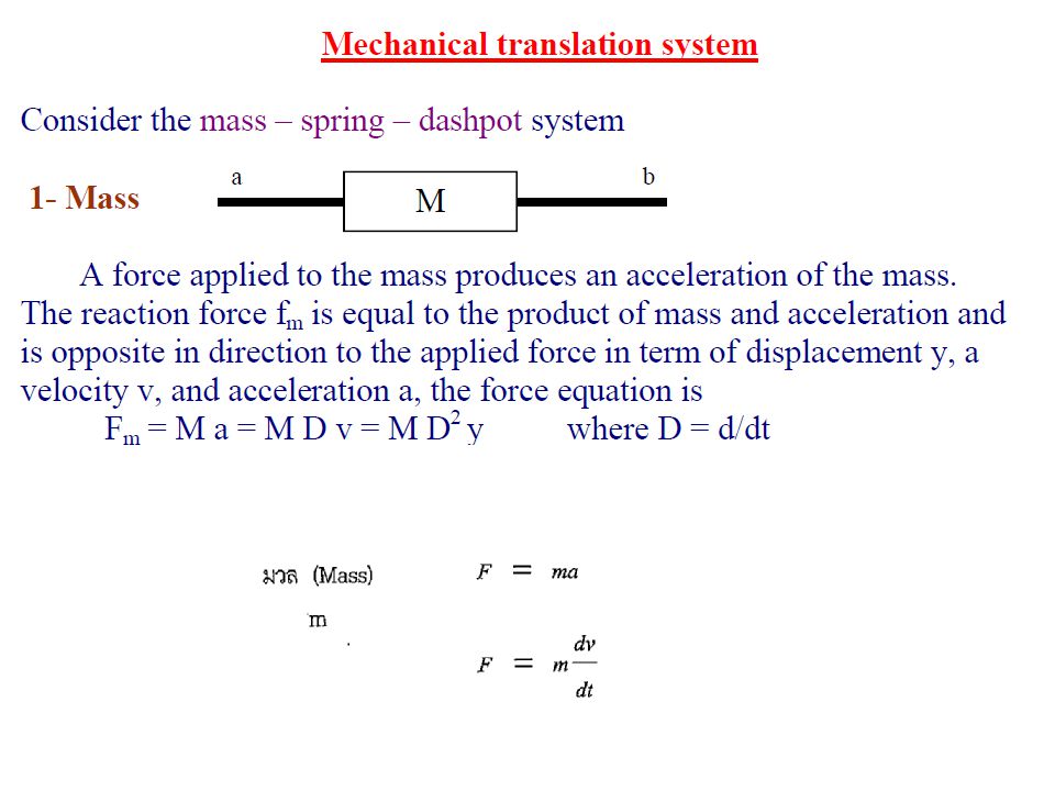
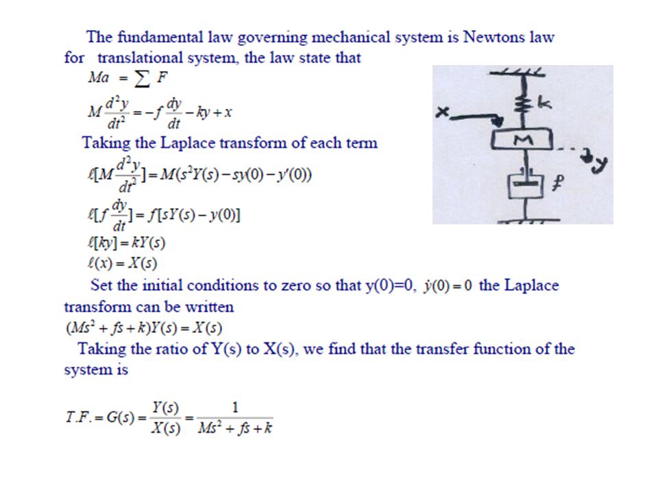
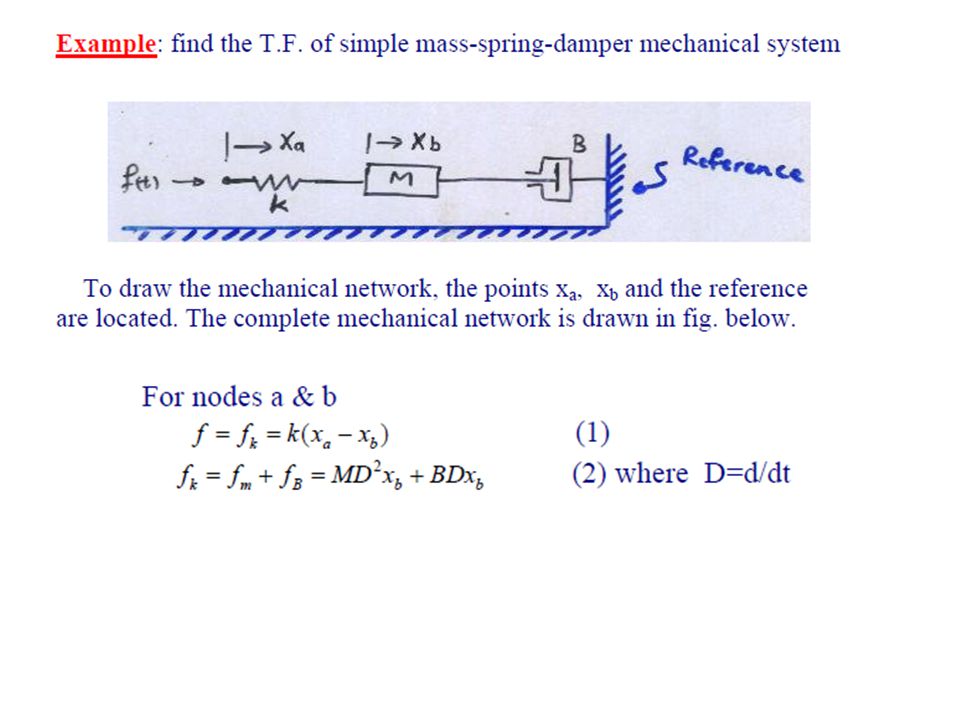
Mechanical, electrical, thermal, hydraulic, economic, biological, etc, systems, may be characterized by differential equations. The response of dynamic system to an input may be obtained if these differential equations are solved. The differential equations can be obtained by utilizing physical laws governing a particular system, for example, Newtons laws for mechanical systems, Kirchhoffs laws for electrical systems, etc.

3
Mathematical models: The mathematical description of the dynamic characteristic of a system The first step in the analysis of dynamic system is to derive its model. Models may assume different forms, depending on the particular system and the circumstances. In obtaining a model, we must make a compromise between the simplicity of the model and the accuracy of results of the analysis. การจำลองระบบด้วยสมการคณิตศาสตร์ (Mathematical Model) โดยทั่วไปจะใช้ วิธีแทนค่าพารามิเตอร์ในระบบด้วยสมการดิฟเฟอร์เรนเชียล จากนั้นใช้การแปลง ลาปลาซ เพื่อหาความสัมพันธ์ระหว่างสมการทางอินพุตกับสมการทางเอาท์พุท ซึ่งอยู่ใน s โดเมน ผลลัพท์จะเรียกว่าทรานเฟอร์ฟังก์ชันและนำผลลัพธ์ที่ได้นี้ไป ใช้ในการวิเคราะห์ระบบต่อไป
 โดยทั่วไปจะใช้ วิธีแทนค่าพารามิเตอร์ในระบบด้วยสมการดิฟเฟอร์เรนเชียล จากนั้นใช้การแปลง ลาปลาซ เพื่อหาความสัมพันธ์ระหว่างสมการทางอินพุตกับสมการทางเอาท์พุท ซึ่งอยู่ใน s โดเมน ผลลัพท์จะเรียกว่าทรานเฟอร์ฟังก์ชันและนำผลลัพธ์ที่ได้นี้ไป ใช้ในการวิเคราะห์ระบบต่อไป.")
4
Linear systems: Linear systems are one in which the equations of the model are linear. A differential equation is linear, if the coefficients are constant or functions only of the independent variable (time). The most important properties of linear system is that the principle of superposition is applicable. In an experimental investigation of dynamic system, if cause and effect are proportional, thus implying that the principle of superposition holds, then the system can be considered linear.
. The most important properties of linear system is that the principle of superposition is applicable. In an experimental investigation of dynamic system, if cause and effect are proportional, thus implying that the principle of superposition holds, then the system can be considered linear..")
5
Linear time invariant systems: the system which represented by differential equation whose coefficients are function of time for example An example of time varying control system is a spacecraft control system. ถ้าค่า a, b, c เป็นค่าคงที่เราเรียกสมการนี้ว่า สมการเชิงเส้นไม่แปรปลี่ยนตาม เวลา (Time Invariant Systems) ถ้าค่า a, b, c เป็นฟังก์ชันหรือแปลงค่าได้ จะเรียกสมการนี้ว่า สมการเชิงเส้น ที่แปรเปลี่ยนตามเวลา (Linear Time Varying Systems)
 ถ้าค่า a, b, c เป็นฟังก์ชันหรือแปลงค่าได้ จะเรียกสมการนี้ว่า สมการเชิงเส้น ที่แปรเปลี่ยนตามเวลา (Linear Time Varying Systems).")
7
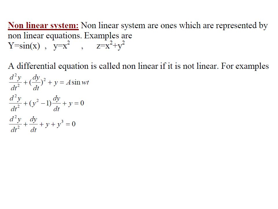
The most important properties of non linear system is that the principle of superposition is not applicable. Because of the mathematical difficulties attached to nonlinear systems, one often it necessary to introduce equivalent linear system which are valid for only a limited range of operation. ( สมการไม่เชิงเส้น แบบอิ่มตัว ) ( สมการไม่เชิง เส้นแบบ มีขอบเขตการ หยุด ) ( สมการไม่เชิง เส้นแบบ กฎกำลังสอง )
 ( สมการไม่เชิง เส้นแบบ มีขอบเขตการ หยุด ) ( สมการไม่เชิง เส้นแบบ กฎกำลังสอง ).")
8
Transfer functions: The transfer function of a linear time-invariant system is define to be the ratio of the Laplace transform (z transform for sample data systems) of the output to the Laplace transform of the input (driving function), under the assumption that all initial conditions are zero. Transfer functions is using for finding a control system stability. It shows the relationship between input and output of “linear time invariant systems” but sometime can be used with linear time varying systems. Transfer functions: the ration of output equation and input equation (already changed to Laplace) under initial condition.
 under initial condition..")
9
Y = output X = input

10
Output Input


.>")


.>")


