STATISTICS FOR AGRICULTURAL RESEARCH สถิติเพื่อการวิจัยทางการเกษตร

งานนำเสนอเรื่อง: "STATISTICS FOR AGRICULTURAL RESEARCH สถิติเพื่อการวิจัยทางการเกษตร"— ใบสำเนางานนำเสนอ:

1 STATISTICS FOR AGRICULTURAL RESEARCH สถิติเพื่อการวิจัยทางการเกษตร
เอกสารประกอบการสอนรายวิชา STATISTICS FOR AGRICULTURAL RESEARCH สถิติเพื่อการวิจัยทางการเกษตร อ.ดร. พัชริน ส่งศรี ภาควิชาพืชศาสตร์และทรัพยากรการเกษตร คณะเกษตรศาสตร์ มหาวิทยาลัยขอนแก่น

2 การวางแผนการทดลองเบื้องต้น
บทที่ 4 การวางแผนการทดลองเบื้องต้น - องค์ประกอบของงานทดลอง - แผนการทดลองแบบสุ่มสมบูรณ์ (CRD) - การวิเคราะห์ความแปรปรวน - การเปรียบเทียบค่าเฉลี่ยเบื้องต้น

3 การทดลอง (experiment)
การแสวงหาคำตอบตามที่ได้วางแผนไว้ เพื่อค้นหาความจริงใหม่ๆ หรือ ทดสอบผลที่ได้ทำมาแล้วว่าเป็นจริงหรือไม่

4 การวิจัยและการทดลอง ความหมายคล้ายกัน แต่การทดลองเป็นระเบียบวิธีวิจัยประเภทหนึ่งในหลายประเภท การวิจัยเชิงประวัติศาสตร์ การวิจัยเชิงพรรณนา การวิจัยเชิงทดลอง

5 สถิติกับการวิจัย

6 สถิติกับการวิจัย วิจัยเป็นการแสวงหาความรู้ใหม่โดยวิธีการทางวิทยาศาสตร์
สถิติเป็นกระบวนการแสวงหาความรู้ใหม่ ที่เกี่ยวกับ การวางแผนการทดลอง การเก็บข้อมูล การวิเคราะห์ข้อมูล การแปรผลข้อมูล ซึ่งจะทำให้ผลการทดลอง หรือ ผลการวิจัยมีความน่าเชื่อถือ

7 ผลการทดลองไม่น่าเชื่อถือ ถ้าหาก
การทดลองขาดการวางแผนการทดลองที่ดี และขาดการเก็บข้อมูลที่ดี ขาดความสมบูรณ์ในการวิเคราะห์ข้อมูลทางสถิติ

8 ดังนั้น นักวิจัยต้องมีความรู้ความเข้าใจเกี่ยวกับสถิติ ก่อนที่จะทำงานวิจัยเรื่องใดเรื่องหนึ่ง

9 หลักการวางแผนการทดลอง
นักวิจัยทำงานทดลอง เพื่อให้ได้ความรู้ใหม่ๆ และนำความรู้นั้น ไปใช้ให้เป็นประโยชน์ เช่น การพัฒนาพันธุ์พืช และ สัตว์ การจัดการดินและน้ำเพื่อเพิ่มผลผลิต

10 หลักการวางแผนการทดลอง
ส่วนประกอบในงานทดลอง ทรีตเมนต์ (treatment) คือ สิ่งหรือวิธีการที่นำมาทดลองเปรียบเทียบกัน หน่วยทดลอง (experimental unit) คือ กลุ่มหรือวัตถุทดลองที่ได้รับทรีตเมนต์ใดทรีตเมนต์หนึ่ง

11 ส่วนประกอบในการทดลอง
ทรีตเมนต์ (treatment) คือ สิ่งทดลองหรือวิธีการ ที่นำมาทดลองเปรียบเทียบกัน เช่น

12 ทรีตเมนต์ (treatment)
วิธีการกำจัดแมลง N0

13 ทรีตเมนต์ (treatment)
พันธุ์พืชที่นำมาทดลองเปรียบเทียบ

14 ทรีตเมนต์ (treatment)
การใช้ปุ๋ยในอัตราต่างๆ

15 2. หน่วยทดลอง (experiment unit) คือกลุ่มของวัตถุทดลองที่ได้รับทรีตเมนต์ใดทรีตเมนต์หนึ่ง เช่น

16 การทดสอบการเปรียบเทียบปุ๋ยสูตรต่างๆ กับต้นหน้าวัวในกระถาง

17 การทดสอบการเปรียบเทียบปุ๋ยสูตรต่างๆ กับต้นหน้าวัวในกระถาง
ปุ๋ยสูตรต่างๆ เป็น tmt กระถาง ต้นหน้าวัวเป็นหน่วยทดลอง

18 การทดลองเปรียบเทียบสูตรอาหารหมู

19 การทดลองเปรียบเทียบสูตรอาหารหมู
อาหารสูตรต่างๆ เป็น tmt หมูในคอกคือ หน่วยการทดลอง

20

21 หลักการวางแผนการทดลอง
ความคลาดเคลื่อนของการทดลอง (Experimental error) ความแตกต่างระหว่างหน่วยทดลองที่ได้รับอิทธิพลของทรีตเมนต์เดียวกัน

22 สาเหตุของความคลาดเคลื่อนของการทดลอง
ความแตกต่างที่มีอยู่ในวัตถุทดลองก่อนการทดลอง (inherent variability)

23 สาเหตุของความคลาดเคลื่อของการทดลอง
1. ความแตกต่างที่มีอยู่ในวัตถุทดลองก่อนการทดลอง (inherent variability) เช่นการทดลองสูตรอาหารต่างๆ กับการเลี้ยงสุกร ปัญหา พันธุกรรมสุกร

24 สาเหตุของความคลาดเคลื่อนของการทดลอง
2. ความแตกต่างเนื่องมาจากสิ่งภายนอก(extraneous variability)

25 สาเหตุของความคลาดเคลื่อนของการทดลอง
2. ความแตกต่างเนื่องมาจากสิ่งภายนอก(extraneous variability) เช่น อิทธิพลของสภาพแวดล้อม การทดลองในสภาพแปลง

26 การทดลองที่มีประสิทธิภาพดี
ต้องมีความคลาดเคลื่อนของการทดลองน้อยที่สุด เท่าที่จะทำได้

27 การลดความคลาดเคลื่อนของการทดลองอันเนื่องมาจากความแตกต่างของวัตถุทดลอง
ทำได้โดยการเลือกวัตถุทดลองให้มีความสม่ำเสมอ หรือเลือกใช้แผนการทดลองที่เหมาะสม

28 สำหรับการลดความคลาดเคลื่อนของการทดลองจากสิ่งภายนอก
โดยทดลองอย่างละมัดระวัง พิถีพิถันในการดูแลงานทดลอง มีความแม่นยำในการใช้เทคนิคในการเก็บข้อมูล มีความรอบคอบในการบันทึกข้อมูล

29 การทำซ้ำ (replication)
คือ การที่ให้ทรีตเมนต์หนึ่งๆ กับหน่วยทดลองอย่างน้อย 2 หน่วยทดลอง เช่น การทดสอบเปรียบเทียบปุ๋ยสองระดับ ได้แก่ 25 กก./ไร่ กับ 50 กก./ไร่ ปลูกทดสอบทั้งหมด 8 แปลง ทรีตเมนต์ละ 4 แปลง (4 ซ้ำ)

30 การทำซ้ำนั้นเป็นสิ่งที่จำเป็นมากในการทำงานทดลอง
เพราะซ้ำนั้น มีบทบาทสำคัญในการทดลองหลายประการ คือ

31 การทำซ้ำ ทำให้ประมาณค่าความคลาดเคลื่อนของการทดลองได้
ความคลาดเคลื่อนของการทดลอง คือความแตกต่างกันของหน่วยทดลองที่ได้รับอิทธิพลของ tmt เดียวกัน ดังนั้นอย่างน้อยต้องมี 2 หน่วยทดลองที่ได้รับอิทธิพลของ tmt เดียวกัน จึงจะประมาณหาค่าความคลาดเคลื่อนของการทดลองได้

32 การทำซ้ำ 2. ทำให้การทดลองมีความเที่ยงตรงมากขึ้นโดยทำให้ standard error ของ treatment mean ลดลง ซึ่งแสดงให้เห็นได้จากสูตร

33 SE = S2/r สูตร เมื่อ SE = standard error ของ treatment mean
S2 = experimental error และ r = จำนวนซ้ำของการทดลอง

34 การทำซ้ำ 3. เป็นการควบคุมความคลาดเคลื่อนของการทดลองได้

35 การทดลองหนึ่ง ๆ จะมีจำนวนซ้ำเท่าใด ขึ้นอยู่กับปัจจัยหลายประการ ได้แก่
1. ความแปรปรวนของลักษณะที่ศึกษา ถ้าความแปรปรวนมาก ควรมีซ้ำมาก แปรปรวนน้อย ซ้ำน้อย 2. จำนวนทรีตเมนต์ - Tmt น้อย ซ้ำมาก เนื่องจากต้องให้มี df ของ error ไม่ควรน้อยกว่า 9 และในช่วงที่เหมาะสมควรจะเป็น 10-12

36 3. ขนาดของความแตกต่าง หมายถึงความแตกต่างระหว่างค่าเฉลี่ยของทรีตเมนต์
ถ้าขนาดความแตกต่างของ tmt มีมาก ไม่ต้องทำซ้ำมาก เช่น การทดสอบวิธีกำจัดวัชพืชกับผลผลิตของข้าวโพดสองการทดลอง 1 เปรียบเทียบวิธีการกำจัดด้วยมือ กับไม่ดายหญ้า 2 เปรียบเทียบวิธีการกำจัดวัชพืชด้วยมือกับสารเคมี 5 สาร การทดลองที่หนึ่งควรมีซ้ำน้อยกว่า

37 การสุ่ม (randomization)
หมายถึง การจัดให้ทรีตเมนต์มีโอกาสที่จะถูกกำหนดให้กับหน่วยทดลองใดเท่าๆ กัน เพื่อที่จะทำให้ทรีตเมนต์อยู่ในหน่วยทดลองใด โดยไม่ลำเอียง (bias) การสุ่มจะทำให้ประมาณค่าความคลาดเคลื่อนของการทดลองได้อย่างถูกต้อง ทำให้การหาค่าเฉลี่ยอิทธิพลของทรีตเมนต์มีความถูกต้อง ทำให้การเปรียบเทียบทรีตเมนต์อยู่บนพื้นฐานของความยุติธรรม

38 ขั้นตอนและสิ่งที่ควรพิจารณาในการวางแผนทำการทดลอง

39 ขั้นตอนและสิ่งที่ควรพิจารณาในการวางแผนทำการทดลอง
ขั้นศึกษาปัญหาและวิเคราะห์ปัญหา ขั้นตั้งวัตถุประสงค์ของการทดลอง ขั้นการเลือกทรีตเมนต์ ขั้นการเลือกวัตถุทดลอง ขั้นการเลือกขนาดการทดลอง ขั้นการเลือกเทคนิคหรือวิธีการ ทดลองที่เหมาะสม ขั้นการเลือกแผนการทดลอง ขั้นการเลือกลักษณะที่ศึกษา และ ลักษณะประกอบอื่น ๆ

40 1. ขั้นศึกษาปัญหาและวิเคราะห์ปัญหา
เช่น การปลูกข้าวโพดมีปัญหาเรื่องโรคทำให้โตไม่ดี การปลูกข้าวมีปัญหาเรื่องดิน การป้องกันการชะช้างของดิน การจะตอบคำถามเหล่านี้ได้จะต้องมีการทดลองเพื่อแก้ปัญหา

41 2. ตั้งวัตถุประสงค์ของการทดลอง
ชัดเจนและเจาะจงว่าจะตอบคำถามอะไร หรือทดสอบสมมุติฐานอะไร ที่สำคัญต้องระบุว่าจะใช้กับประชากรกลุ่มป้าหมายประชากรใด เช่น งานทดลองหนึ่ง มีวัตถุประสงค์เพื่อหาอัตราปุ๋ยที่เหมาะสมต่อการปลูกข้าวนาปรังในเขตชลประทานภาคกลาง ดังนั้นงานทดลองนี้ใช้ได้กับเฉพาะที่ทดลองเท่านั้น

42 3. การเลือกทรีตเมนต์ ต้องพิจารณาว่า tmt ที่เลือกนั้น สามารถทำให้บรรลุวัตถุประสงค์ของการทดลองหรือสามารถตอบคำถามที่ตั้งเอาไว้ได้ เช่น ปัญหา ข้าวผลผลิตต่ำ นักวิจัยจึงตั้งสมมุติฐานสองอัน ดังนี้ วัชพืช? หากเป็นวัชพืชหามีวิธีการกำจัดอย่างไร 1. tmt ควรเป็น กำจัดวัชพืช กับ ไม่กำจัด 2. tmt ควรมีหลายวิธี เช่นใช้แรงงานคนกับสารเคมี

43 4. การเลือกวัตถุทดลอง วัตถุทดลองควรมีความสม่ำเสมอหรือมีความแปรปรวนน้อย เพราะจะทำให้ความคลาดเคลื่อนของการทดลองน้อยด้วย

44 5. การเลือกขนาดการทดลอง
เล็กใหญ่ ขึ้นกับ tmt ซ้ำ และขนาดของหน่วยทดลอง จำนวน tmt ขึ้นกับ วัตถุประสงค์ของการทดลองด้วย จำนวนซ้ำ ขึ้นกับ ความแปรปรวนของลักษณะที่ศึกษา จำนวน tmt ขนาดของความแตกต่างของ tmt

45 6. ขั้นการเลือกเทคนิคหรือวิธีการทดลองที่เหมาะสม
ควรควบคุมอิทธิพลจากภายนอกเพียงพอให้ tmt แสดงอิทธิพลได้ในสภาพที่เหมือนกัน 7. ขั้นเลือกแผนการทดลอง 8. เลือกลักษณะที่ศึกษา

46 แผนการทดลองแบบ Completely Randomized Design (CRD)

47 ใช้ในกรณีที่หน่วยทดลองมีความสม่ำเสมอเหมือนกัน
สามารถที่จะควบคุมสภาพแวดล้อมให้หน่วยทดลองมีความเหมือนกันได้

48 งานทดลองในกระถาง

49 งานทดลองในห้องปฏิบัติการ

50 การสุ่ม (randomization)
คือการสุ่มทรีตเมนต์สำหรับหน่วยทดลอง เป็นลักษณะของการสุ่มแบบสมบูรณ์ ทุกๆ หน่วยทดลองมีโอกาสที่จะได้รับทรีตเมนต์ใดทรีตเมนต์หนึ่งอย่างยุติธรรม

51 สมมติว่างานทดลองหนึ่ง
ต้องการเปรียบเทียบทรีตเมนต์ 4 ทรีทเมนต์ คือ A B C และ D แต่ละทรีตเมนต์มี 5 ซ้ำ

52 ขั้นตอนการสุ่มมีดังนี้
ขั้นที่ 1 กำหนดหน่วยทดลองที่ต้องใช้ทั้งหมด ซึ่งจะเท่ากับ จำนวนทรีตเมนต์ (4) คูณด้วยจำนวนซ้ำ (5) D A C C A B B D B A D D B C A B C D A C

53 ขั้นที่ 2 การให้เบอร์ของหน่วยทดลอง เพื่อการสะดวก ในการ
สุ่มจะให้เบอร์ของหน่วยทดลองตั้งแต่ 1 ถึง n คือจำนวนหน่วยทดลองทั้งหมด จากตัวอย่างจะได้ เบอร์หน่วยทดลองตั้งแต่ 1 ถึง 20 ดังนี้

54 1 2 3 4 5 6 7 8 9 10 11 12 13 14 15 16 17 18 19 20

55 จับฉลาก หรือใช้ตารางเลขสุ่ม
ขั้นที่ 3 สุ่มจัดหน่วยทดลองให้ได้รับทรีตเมนต์ต่าง ๆ โดยวิธี จับฉลาก หรือใช้ตารางเลขสุ่ม

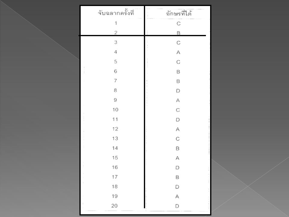
56 1. การสุ่มโดยการจับฉลาก
ทำฉลากที่เหมือน ๆ กันจำนวน 20 ใบ เขียน ทรีตเมนต์ลงบนฉลาก ทรีตเมนต์ละ 5 ใบตามจำนวนซ้ำ เขียน A B C และ D ลงบนฉลากอย่างละ 5 แผ่น ม้วนฉลากให้เหมือนกัน โดยไม่ให้เห็นตัวอักษรทรีตเมนต์ที่เขียนอยู่ภายใน ใส่ฉลากลงในกล่องเขย่าให้ปนกันดีแล้วค่อย ๆ จับฉลากขึ้นมาทีละแผ่น โดยไม่ใส่ฉลากกลับคืน แผ่นแรกได้

57 B C A D D B C A C D A B C D B A A D B C

58 อักษรใดก็จะเป็นทรีตเมนต์สำหรับหน่วยทดลองที่ 1 แผ่นที่ 2 ได้อักษรใดก็เป็นทรีตเมนต์สำหรับหน่วยทดลองที่ 2 ทำเช่นนี้จนครบ 20 แผ่นดังตาราง

59

60 แผนผังการทดลอง (lay out)
คือแผนผังที่แสดงตำแหน่งของหน่วยทดลองในการทดลอง แต่ละหน่วยทดลองมีการระบุทรีตเมนต์ที่ได้รับจากการสุ่มไว้อย่างชัดเจน อำนวยความสะดวกให้กับผู้ทดลอง ในการให้ทรีตเมนต์กับหน่วยทดลองต่าง ๆ ได้อย่างถูกต้อง

61 1 C 2 B 3 C 4 A 5 C 6 B 7 B 8 D 9 A 10 C 11 D 12 A 13 C 14 B 15 A 16 D 17 B 18 D 19 A 20 D

62 ตัวอย่าง นักวิชาการเกษตรทำการทดลองหาสูตรดินผสมที่เหมาะสมสำหรับการปลูกกุหลาบ คัดเลือกกิ่งตอนกุหลาบที่มีอายุและขนาดกิ่งที่เท่ากัน นำมาปลูกในกระถางที่บรรจุสูตรดิน A B C และ D (ทำ 4 ซ้ำ) หลังจากปลูกได้ 60 วัน วัดความสูงของต้นกุหลาบหน่วยทดลองได้ดังนี้

63 1 A 58 2 B 31 3 C 31 4 A 82 5 C 65 6 D 108 7 B 53 8 D 99 9 A 89 10 C 33 11 D 126 12 B 44 13 C 43 14 B 22 15 A 72 16 D 147

64 ตารางแจกแจงข้อมูล หลังจากที่วัดข้อมูลจากหน่วยทดลองแต่ละหน่วยแล้ว เพื่อความสะดวกในการวิเคราะห์ข้อมูล ควรนำตัวเลขข้อมูลจัดเรียงในตาราง

65 ความสูง (เซ็นติเมตร) A B C D 58 31 65 108 89 22 43 126 72 53 33 99 82
44 147 ผลรวม Yi. = 301 150 172 480 ค่าเฉลี่ย = 75.25 37.50 120 Grand total = 1103 Grand mean = 68.94

66 จากตารางจะเห็นได้ว่าการเรียงตัวเลขจะเอาเลขไหนขึ้นก่อนหลังก็ได้
แต่ต้องเป็นตัวเลขที่ได้จากหน่วยทดลองที่ได้รับอิทธิพลทรีตเมนต์เดียวกันไว้ด้วยกัน หรือจัดแบ่งข้อมูลตามทรีตเมนต์นั่นเอง ลักษณะการจัดข้อมูลตามทรีตเมนต์อย่างเดียว เรียกข้อมูลนี้ว่ามีการแจกแจงแบบทางเดียว (one-way classification) คือแจกแจงตามทรีตเมนต์เพียงอย่างเดียว

67 สัญลักษณ์ที่ใช้แทนข้อมูล
ถ้าให้ Yij คือข้อมูลที่ได้จากหน่วยทดลองที่ j ในทรีตเมนต์ที่ i เมื่อ i = 1, 2,…….t และ j = 1, 2,…..r โดย t คือจำนวนทรีตเมนต์ r คือจำนวนซ้ำ ดังนั้นข้อมูลในตารางสามารถเขียนเป็นสัญลักษณ์ได้ดังนี้

68 สูตรดินผสม A B C D Y11 Y21 Y31 Y41 Y12 Y22 Y32 Y42 Y13 Y23 Y33 Y43 Y14 Y24 Y34 Y44 ผลรวม Yi. Y1. Y2. Y3. Y4. Y.. = Grand total ค่าเฉลี่ย Yi Y.. = Grand mean

69 การวิเคราะห์ข้อมูล การวิเคราะห์ข้อมูลที่ได้จากการศึกษา โดยใช้แผนการทดลองแบบ CRD มีรูปแบบตารางการวิเคราะห์ข้อมูล ในรูปของการวิเคราะห์ความแปรปรวน (Analysis of Variance : ANOVA)

70 t = จำนวนทรีตเมนต์, r = จำนวนซ้ำ N = จำนวนหน่วยทดลองทั้งหมด = tr
สูตรที่ใช้ในการคำนวณดังนี้ Source of variation (SOV) Degree of freedom Sum of Square (S.S.) Mean Squares (M.S.) Treatment (t-1) iY2i. – (Y..)2 Treatment S.S. Error t(r-1) Total S.S. – treatment S.S Error S.S. Total N-1 ijY2ij–(Y..) 2 r tr t - 1 t (r- 1) tr t = จำนวนทรีตเมนต์, r = จำนวนซ้ำ N = จำนวนหน่วยทดลองทั้งหมด = tr

71 ขั้นตอนวิธีการคำนวณและทดสอบทางสถิติ
การคำนวณค่า degree of freedom (df) คำนวณค่า Correction factor (C.F.) คำนวณค่า Sum of Squares (S.S.) คำนวณค่า Mean Squares (M.S.) คำนวณค่า F- Value นำค่าที่คำนวณได้ไปใส่ในตารางวิเคราะห์ความแปรปรวน (ANOVA) คำนวณค่า Coefficient of variation (C.V.) การทดสอบทางสถิติ

72 1

73 ขั้นตอนวิธีการคำนวณและทดสอบทางสถิติ
การคำนวณค่า degree of freedom (df) ค่า df ของ Total คำนวณจาก tr-1 = (4 x 4)-1 = 15 ค่า df ของ Treatment คำนวณจาก t-1 = 4-1 = 3 ค่า df ของ Error คำนวณจาก t(r-1) = 4(4-1) = 12

74 2

75 2. คำนวณค่า Correction factor (C.F.)
C.F. = (Y..)2 tr = (1103)2 (4)(4) =

76 3

77 3. คำนวณค่า Sum of Squares (S.S.)
Total S.S. = ijY2ij – C.F. = ( …… ) –76,038.06 = 96,457 –76,038.06 = 20,418.94 น้ำหนัก (กรัม) A B C D 58 31 65 108 89 22 43 126 72 53 33 99 82 44 147 ผลรวม Yi. = 301 150 172 480 ค่าเฉลี่ย = 75.25 37.50 120

78 Treatment S.S. = iY2i. – C.F. r = ( ) –76,038.06 4 = 93, –76,038.06 = 17,233.19 น้ำหนัก (กรัม) A B C D 58 31 65 108 89 22 43 126 72 53 33 99 82 44 147 ผลรวม Yi. = 301 150 172 480 ค่าเฉลี่ย = 75.25 37.50 120

79 Error S.S. = Total S.S. – Treatment S.S.
= 20, – 17,233.19 = 3,185.75

80 4

81 4. คำนวณค่า Mean Squares (M.S.) Treatment M.S. = Treatment S.S.
= 17,233.19 3 = 5, Error M.S. = Error S.S. t(r-1) = 3,185.75 12 =

82 5

83 5. คำนวณค่า F- Value F = Treatment M.S. = 5,744.39 = 21.64 Error M.S.
265.48 = 21.64

84 6

85 6. นำค่าที่คำนวณได้ไปใส่ในตารางวิเคราะห์ความแปรปรวน (ANOVA)

86 ตารางวิเคราะห์ความแปรปรวน (ANOVA)
SOV df S.S. M.S. F Treatment 3 17,233.19 5,744.39 21.64 Error 12 3,185.75 265.48 Total 15 20,418.94

87 7

88 7. คำนวณค่า Coefficient of variation (C.V.)
C.V. = Error M.S. x 100 Y.. =  x 100 68.94 = %

89 ค่า C.V. เป็นตัวเลขดัชนีบอกความเที่ยงตรงของงานทดลอง

90 8

91 8. การทดสอบทางสถิติ การทดสอบทางสถิติเพื่อทดสอบว่าอิทธิพล TMT ที่ศึกษาแตกต่างกันหรือไม่ โดยการเปิดตาราง F ที่ df ของ Treatment และ df ของ Error และจะต้องกำหนดระดับความเชื่อมั่นที่ใช้ทดสอบ

92 ถ้าค่า F ที่ได้จากการคำนวณสูงกว่าค่า F ที่ได้จากการเปิดตารางที่ P = 0
ถ้าค่า F ที่ได้จากการคำนวณสูงกว่าค่า F ที่ได้จากการเปิดตารางที่ P = 0.05 แสดงว่า TMT ที่นำมาเปรียบเทียบมีความแตกต่างกันอย่างมีนัยสำคัญทางสถิติที่ระดับความเชื่อมั่น 95 % ซึ่งจะใส่เครื่องหมาย * ไว้ เหนือค่า F ในตาราง ANOVA

93 ถ้าค่า F ที่ได้จากการคำนวณสูงกว่าค่า F ที่ได้จากการเปิดตารางที่ P = 0
แสดงว่า TMT ที่นำมาเปรียบเทียบมีความแตกต่างกันอย่างมีนัยสำคัญทางสถิติที่ระดับความเชื่อมั่น 99 % ซึ่งจะใส่เครื่องหมาย ** ไว้ เหนือค่า F ในตาราง ANOVA

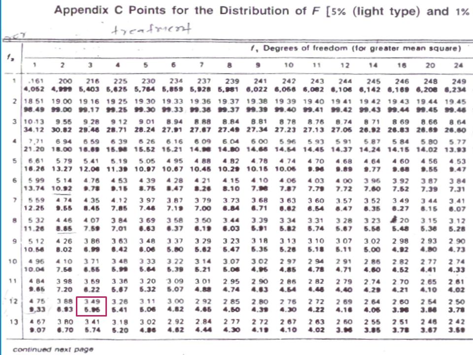
94 เปิดตาราง df ของ Treatment df ของ Error F ที่คำณวณได้

95

96 ตารางวิเคราะห์ความแปรปรวน (ANOVA)
SOV df S.S. M.S. F Treatment 3 17,233.19 5,744.39 21.64** Error 12 3,185.75 265.48 Total 15 20,418.94 CV (%) = %

97 การทดสอบความแตกต่างระหว่าง TMT ที่ศึกษา
โดยใช้ค่า F นั้นเป็นการทดสอบความแตกต่างของ TMT ทั้งกลุ่มที่ศึกษาว่ามีความแตกต่างกันหรือไม่ แต่ไม่สามารถบอกได้ว่าค่าเฉลี่ยของทรีตเมนต์ใดแตกต่างจากทรีตเมนต์ใดบ้าง ในทางปฏิบัติมักจะต้องเปรียบเทียบค่าเฉลี่ยระหว่าง TMT

98 การเปรียบเทียบค่าเฉลี่ย

99 วิธีการเปรียบเทียบค่าเฉลี่ยของทรีตเมนต์
นิยมใช้มากที่สุดในการทดลองทางการเกษตร คือ Least significant difference (LSD) Duncan’s multiple range test (DMRT)

100 การเปรียบเทียบค่าเฉลี่ย ด้วยวิธี LSD

101 การเปรียบเทียบค่าเฉลี่ยด้วยวิธี LSD
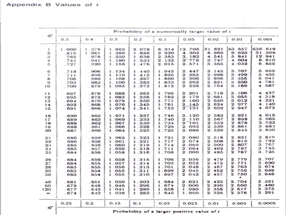
LSD = t 2Error M.S. r เมื่อ t คือ ค่า t จากตาราง t (two-tailed) ที่ df ของ Error และ P =  จากตารางจะเปรียบเทียบค่าเฉลี่ยของทรีตเมนต์ที่ระดับความเชื่อมั่น 99 % (P = 0.01)

102

103 LSD0.01 = 3.05 2 x 4 =

104 2. คำนวนแตกต่างระหว่างค่าเฉลี่ยของคู่ทรีตเมนต์ที่ต้องการเปรียบเทียบ

105 ค่าความแตกต่างระหว่าง A กับ B = 75.25 – 37.50
= 37.75 ค่าความแตกต่างระหว่าง A กับ C = – 43.00 = 32.25 ค่าความแตกต่างระหว่าง A กับ D = – 120.0 = ค่าความแตกต่างระหว่าง B กับ C = – 43.00 = -5.5 ค่าความแตกต่างระหว่าง B กับ D = – = ค่าความแตกต่างระหว่าง C กับ D = – = -77

106 เมื่อ A, B, C, และ D คือทรีตเมนต์ สูตรดิน 4 สูตร
จำนวนคู่ที่เปรียบเทียบกันได้สูงสุด = t(t-1) /2 คู่ เมื่อ t คือจำนวนทรีตเมนต์ที่ศึกษา

107 3. นำค่าความแตกต่างระหว่างคู่ของ TMT ที่ต้องการเปรียบเทียบมาเทียบค่า LSD ที่คำนวณได้

108 37.75 35.19 32.25 44.75 5.5 82.5 77.0 TMTเปรียบเทียบ ค่าต่างระหว่างคู่
ค่า LSD ข้อสรุป A กับ B 37.75 35.19 A กับ C 32.25 A กับ D 44.75 B กับ C 5.5 B กับ D 82.5 C กับ D 77.0

109 37.75 35.19 แตกต่าง 32.25 44.75 5.5 82.5 77.0 TMTเปรียบเทียบ
ค่าต่างระหว่างคู่ ค่า LSD ข้อสรุป A กับ B 37.75 35.19 แตกต่าง A กับ C 32.25 A กับ D 44.75 B กับ C 5.5 B กับ D 82.5 C กับ D 77.0

110 TMTเปรียบเทียบ ค่าต่างระหว่างคู่ ค่า LSD ข้อสรุป A กับ B 37.75 35.19 แตกต่าง A กับ C 32.25 ไม่แตกต่าง A กับ D 44.75 B กับ C 5.5 B กับ D 82.5 C กับ D 77.0

111 TMTเปรียบเทียบ ค่าต่างระหว่างคู่ ค่า LSD ข้อสรุป A กับ B 37.75 35.19 แตกต่าง A กับ C 32.25 ไม่แตกต่าง A กับ D 44.75 B กับ C 5.50 B กับ D 82.50 C กับ D 77.0

112 4. แสดงผลการทดสอบทางสถิติ
TMTเปรียบเทียบ ค่าต่างระหว่างคู่ ค่า LSD ข้อสรุป A กับ B 37.75 35.19 แตกต่าง A กับ C 32.25 ไม่แตกต่าง A กับ D 44.75 B กับ C 5.50 B กับ D 82.50 C กับ D 77.0

113 น้ำหนักเฉลี่ย (กรัม) 120.0 75.25 43.00 37.50 D A C B 37.75 35.19
TMTเปรียบเทียบ ค่าต่างระหว่างคู่ ค่า LSD ข้อสรุป A กับ B 37.75 35.19 แตกต่าง A กับ C 32.25 ไม่แตกต่าง A กับ D 44.75 B กับ C 5.50 B กับ D 82.50 C กับ D 77.0 น้ำหนักเฉลี่ย (กรัม) D 120.0 A 75.25 C 43.00 B 37.50

114 ตัวอักษรเหมือนกันเพียงตัวเดียวถือว่าไม่ต่างกัน
น้ำหนักเฉลี่ย (กรัม) D 120.0a A 75.25b C 43.00bc B 37.50c ตัวอักษรเหมือนกันเพียงตัวเดียวถือว่าไม่ต่างกัน

115 ตารางสรุป ตัวอักษรเหมือนกันเพียงตัวเดียวถือว่าไม่ต่างกัน สูตรดิน
ความสูงเฉลี่ย (กรัม) A 75.25b B 37.50c C 43.00bc D 120.0a ตัวอักษรเหมือนกันเพียงตัวเดียวถือว่าไม่ต่างกัน

116 การเปรียบเทียบค่าเฉลี่ยโดยวิธี LSD นั้นเป็นวิธีที่ง่าย และสะดวกในการใช้
ข้อจำกัดในการใช้คือเหมาะที่ใช้กับการเปรียบเทียบในการศึกษาที่มี TMT ไม่มากนัก

117 การเปรียบเทียบค่าเฉลี่ยด้วยวิธี DMRT

118 การเปรียบเทียบค่าเฉลี่ยด้วยวิธี DMRT
ซับซ้อนมากกว่า LSD แต่การใช้ DMRT จะใช้ได้ดีแม้มี TMT ที่ศึกษาเป็นจำนวนมาก (ข้อจำกัดของวิธี LSD) การใช้ DMRT ในการเปรียบเทียบนั้นมีค่าวิกฤติในการเปรียบเทียบมากกว่า 1 ค่า (วิธี LSD ที่มีค่าวิกฤติเพียงค่าเดียว)

119 ขั้นตอนการคำนวณ น้ำหนักเฉลี่ย (g) ลำดับที่ 120.0 1 75.25 2 43.00 3
1. เรียงลำดับค่าเฉลี่ยของ TMT จากน้อยไปหามาก หรือจากมากไปหาน้อย TMT น้ำหนักเฉลี่ย (g) ลำดับที่ D 120.0 1 A 75.25 2 C 43.00 3 B 37.50 4

120 2. คำนวณค่า standard error ของค่าเฉลี่ย (Syi.)
Syi. = Error M.S. / r =  / 4 = 8.15

121 3. คำนวณค่า shortest significant ranges สำหรับใช้เปรียบเทียบค่าเฉลี่ยที่ได้เรียงลำดับไว้ ที่ระดับความเชื่อมั่นที่ต้องการ จากสูตร Rp = rpSyi. ค่า rp คือ significant studentized range ซึ่งได้จากการเปิดตาราง ที่ระดับความเชื่อมั่นที่ต้องการ ค่า df ที่ใช้คือ df ของ error, p = 2, 3,4,……t เมื่อ t คือ จำนวนทรีตเมนต์ได้ค่า rp และคำนวณค่า Rp ได้ดังตาราง

122 4.32 4.55 4.68

123 rp (0.01) จากตาราง Rp (จากการคำนวณ) 4.32 (8.15 x 4.23) = 34.47 4.55
4.68 (8.15 x 4.68) = 38.14

124 4. ทดสอบความแตกต่างระหว่างค่าเฉลี่ยของ TMT ที่ได้รับจากการลำดับที่ไว้ทีละคู่

125 ลำดับที่เปรียบเทียบ TMT ที่เปรียบเทียบ ผลต่างของค่าเฉลี่ย ค่า P ค่า Rp ข้อสรุป 1 กับ 2 D กับA 44.75 2 34.47 1 กับ 3 D กับ C 77.00 3 37.08 1 กับ 4 D กับ B 82.50 4 38.14 2 กับ 3 A กับ C 32.25 2 กับ 4 A กับ B 37.75 3 กับ 4 C กับB 5.50

126 ลำดับที่เปรียบเทียบ TMT ที่เปรียบเทียบ ผลต่างของค่าเฉลี่ย ค่า P ค่า Rp ข้อสรุป 1 กับ 2 D กับA 44.75 2 34.47 แตกต่าง 1 กับ 3 D กับ C 77.00 3 37.08 1 กับ 4 D กับ B 82.50 4 38.14 2 กับ 3 A กับ C 32.25 2 กับ 4 A กับ B 37.75 3 กับ 4 C กับB 5.50

127 ลำดับที่เปรียบเทียบ TMT ที่เปรียบเทียบ ผลต่างของค่าเฉลี่ย ค่า P ค่า Rp ข้อสรุป 1 กับ 2 D กับA 44.75 2 34.47 แตกต่าง 1 กับ 3 D กับ C 77.00 3 37.08 1 กับ 4 D กับ B 82.50 4 38.14 2 กับ 3 A กับ C 32.25 2 กับ 4 A กับ B 37.75 3 กับ 4 C กับB 5.50

128 ลำดับที่เปรียบเทียบ TMT ที่เปรียบเทียบ ผลต่างของค่าเฉลี่ย ค่า P ค่า Rp ข้อสรุป 1 กับ 2 D กับA 44.75 2 34.47 แตกต่าง 1 กับ 3 D กับ C 77.00 3 37.08 1 กับ 4 D กับ B 82.50 4 38.14 2 กับ 3 A กับ C 32.25 ไม่แตกต่าง 2 กับ 4 A กับ B 37.75 3 กับ 4 C กับB 5.50

129 5. แสดงผลการทดสอบทางสถิติ
นิยมเขียนตัวอักษรกำกับไว้เหนือตัวเลขค่าเฉลี่ยของแต่ละทรีตเมนต์ ค่าเฉลี่ยของทรีตเมนต์ที่ไม่แตกต่างกันจะถูกกำกับด้วยตัวอักษรที่เหมือนกัน

130 น้ำหนักเฉลี่ย (กรัม) 120.00 75.25 43.00 37.50 ทรีตเมนต์ลำดับที่ 1 D 2
ลำดับที่เปรียบเทียบ TMT ที่เปรียบเทียบ ผลต่างของค่าเฉลี่ย ค่า P ค่า Rp ข้อสรุป 1 กับ 2 D กับA 44.75 2 34.47 แตกต่าง 1 กับ 3 D กับ C 77.00 3 37.08 1 กับ 4 D กับ B 82.50 4 38.14 2 กับ 3 A กับ C 32.25 ไม่แตกต่าง 2 กับ 4 A กับ B 37.75 3 กับ 4 C กับB 5.50 ทรีตเมนต์ลำดับที่ น้ำหนักเฉลี่ย (กรัม) 1 D 120.00 2 A 75.25 3 C 43.00 4 B 37.50

131 น้ำหนักเฉลี่ย (กรัม) 120.00a 75.25b 43.00bc 37.50c
ทรีตเมนต์ลำดับที่ น้ำหนักเฉลี่ย (กรัม) 1 D 120.00a 2 A 75.25b 3 C 43.00bc 4 B 37.50c

132 เอกสารอ่านเพิ่มเติม สนั่น จอกลอย 2535 สถิติเพื่อการวิจัยทางการเกษตร
Gomez, K.A. and A.A. Gomez Statistical procedures for agricultural research.

133 บทที่ 5 การวิเคราะห์ความสัมพันธ์ทางสถิติ
บทที่ 5 การวิเคราะห์ความสัมพันธ์ทางสถิติ - การวิเคราะห์ค่าสหสัมพันธ์ - การสร้างสมการทำนายอย่างง่าย

134 Introduction to Correlation and Regression
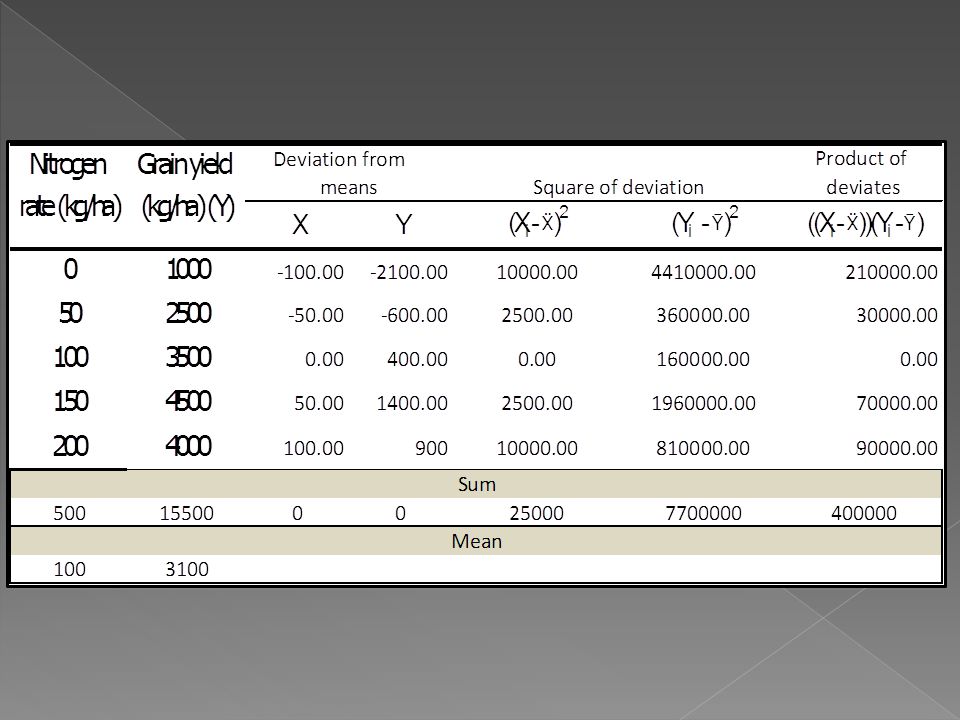
Dr. Patcharin Songsri Dept. Plant Sci. & Agric Resources, Fact. Agriculture, Khon Kaen University

135 Chapter Goals After completing this chapter, you should be able to:
Calculate and interpret the simple correlation between two variables Determine whether the correlation is significant Calculate and interpret the simple linear regression equation for a set of data Understand the assumptions behind regression analysis Determine whether a regression model is significant

136 Correlation

137 Correlation Pearson correlation coefficient (r) measures the degree of linear association between two intervally scaled variables

138 Correlation Two pieces of information:
The strength of the relationship The direction of the relationship

139 Correlation (direction)
Positive correlation: high values of one variable associated with high values of the other Example: Higher STAT scores are associated with better grades in the first year of college

140 Correlation (direction)
Negative correlation: high values of one variable associated with low values of the other Example: reduced in fruit number is related with Increased in fruit size

141 Correlation Correlation Example (positive correlation)
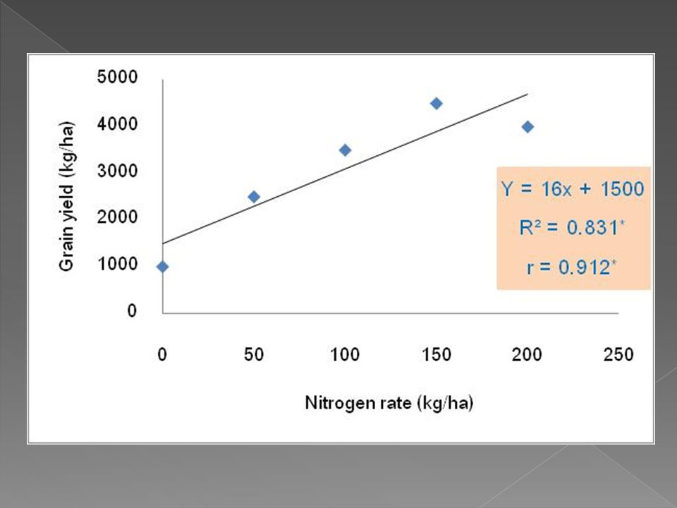
A measure of association between two numerical variables. Example (positive correlation) Typically, in the summer as the temperature increases people are thirstier. Typically, in the summer as the temperature increases people are thirstier. Consider the two numerical variables, temperature and water consumption. We would expect the higher the temperature, the more water a given person would consume. Thus we would say that in the summer time, temperature and water consumption are positively correlated.

142 How would you describe the graph?
This graph helps us visualize what appears to be a somewhat linear relationship between temperature and the amount of water one drinks.

143 How “strong” is the linear relationship?

144 Direction of Association
Positive Correlation Negative Correlation Direction of the Association: The association can be either positive or negative. Positive Correlation: as the x variable increases so does the y variable. Example: In the summer, as the temperature increases, so does thirst. Negative Correlation: as the x variable increases, the y variable decreases. Example: As the price of an item increases, the number of items sold decreases.

145 Other Strengths of Association

146 Strength of Linear Association

147 Examples of Approximate r Values
y x r = -1 r = -0.6 r = 0

148 Strength of Linear Association
r value Interpretation 1 perfect positive linear relationship no linear relationship -1 perfect negative linear relationship Strength of the Association:  The strength of the linear association is measured by the sample Correlation Coefficient, r.  r can be any value from –1 to +1.    The closer r is to one (in magnitude) the stronger the linear association.   If r equals zero, then there is no linear association between the two variables. 

149 Other Strengths of Association
r value (+,-) Interpretation strong association moderate association > 0.4 weak association *  No other values of r have precise definitions of strength. See the chart below. Note:  All of the values in the second table are positive. Thus the associations are positive. The same strength interpretations hold for negative values of r, only the direction interpretations of the association would change.

150 Measuring the Relationship
Pearson’s Sample Correlation Coefficient, r measures the direction and the strength of the linear association between two numerical paired variables.

151 the Correlation Coefficient (r)
Calculating the Correlation Coefficient (r)

152

153 Compute the Correlation Coefficient (r)

154 r =0.91*

155 Reminder Correlation does not imply a causal relationship between variables Causal inferences are made based on underlying knowledge and theories Correlations can be affected by outliers (which is why scatter plots are useful) Underlying relationship is assumed to be linear

156 The Correlation Coefficient
• The strength of a linear relationship is measured by the correlation coefficient • The sample correlation coefficient is given the symbol “r”

157 Fundamental Rule of Correlation
• Correlation DOES NOT imply causation – Just because two variables are highly correlated does not mean that the explanatory variable “causes” the Response

158 Cautions • The correlation coefficient (r) only gives us an indication about the strength of a linear relationship. • Two variables may have a strong curvilinear relationship, but they could have a “weak” value for ‘r’

159 Regression

160 Regression Regression
Specific statistical methods for finding the “line of best fit” for one response (dependent) numerical variable based on one or more explanatory (independent) variables.

161 Curve Fitting vs. Regression
Includes using statistical methods to assess the "goodness of fit" of the model.  (ex. Correlation Coefficient)

162 Regression: 3 Main Purposes
To describe (or model) To predict (or estimate) To control (or administer) To describe or model a set of data with one dependent variable and one (or more) independent variables. To predict or estimate the values of the dependent variable based on given value(s) of the independent variable(s). To control or administer standards from a useable statistical relationship.

163 Simple Linear Regression
Statistical method for finding the “line of best fit” for one response (dependent) numerical variable based on one explanatory (independent) variable.   Simple: only one independent variable Linear in the Independent Variable:  the independent variable only appears to the first power.

164 Steps to Reaching a Solution
Draw a scatter plot of the data. Visually, consider the strength of the linear relationship.

165 Steps to Reaching a Solution
Draw a scatter plot of the data. Visually, consider the strength of the linear relationship. If the relationship appears relatively strong, find the correlation coefficient as a numerical verification.

166 Steps to Reaching a Solution
Draw a scatter plot of the data. Visually, consider the strength of the linear relationship. If the relationship appears relatively strong, find the correlation coefficient as a numerical verification. If the correlation is still relatively strong, then find the simple linear regression line.

167 Coefficient of Determination, R2
The coefficient of determination is the portion of the total variation in the dependent variable that is explained by variation in the independent variable The coefficient of determination is also called R-squared and is denoted as R2 where

168 Coefficient of Determination, R2
(continued) Coefficient of determination Note: In the single independent variable case, the coefficient of determination is where: R2 = Coefficient of determination r = Simple correlation coefficient

169 Examples of Approximate R2 Values
y R2 = 1 Perfect linear relationship between x and y: 100% of the variation in y is explained by variation in x x R2 = 1 y x R2 = +1

170 Examples of Approximate R2 Values
y 0 < R2 < 1 Weaker linear relationship between x and y: Some but not all of the variation in y is explained by variation in x x y x

171 Examples of Approximate R2 Values
y No linear relationship between x and y: The value of Y does not depend on x. (None of the variation in y is explained by variation in x) x R2 = 0

172 Example Temperature (F) Water Consumption (ounces) 75 16 83 20 85  25 85 27 92 32 97 48 99

173 Interpreting and Visualizing
Interpreting the result: y = bx + c The value of b is the slope The value of c is the y-intercept r is the correlation coefficient r2 is the coefficient of determination

174 Interpreting and Visualizing
Write down the equation of the line in slope intercept form. Press Y= and enter the equation under Y1. (Clear all other equations.)  Press GRAPH and the line will be graphed through the data points.

175 Interpretation in Context
Regression Equation: y=1.5*x Water Consumption = 1.5*Temperature

176 Interpretation in Context
Slope = 1.5 (ounces)/(degrees F) for each 1 degree F increase in temperature, you expect an increase of 1.5 ounces of water drank.

177 Interpretation in Context
y-intercept = -96.9 For this example, when the temperature is 0 degrees F, then a person would drink about -97 ounces of water. That does not make any sense! Our model is not applicable for x=0.   And we cannot expect it be accurate at such low temperatures, because the sample of data was taken in the summer time and the temperatures range from 75 to 99 degrees Fahrenheit. Thus the model only predicts for temperatures in approximately that range. 

178 Prediction Example Predict the amount of water a person would drink when the temperature is 95 degrees F. Solution: Substitute the value of x=95 (degrees F) into the regression equation and solve for y (water consumption). If x=95, y=1.5* = 45.6 ounces.   Solution: Substitute the value of x=95 (degrees F) into the regression equation y=1.5*x   and solve for y (water consumption). y=1.5*x if x=95, then y=1.5* = 45.6 ounces.   Note: Since 95 degrees F is in the range of values that were used to find the regression equation, then we can use this equation to predict the water consumption. If the desired prediction had been for 50 degrees F, then the model should not be used, since the value of x does not fall in the range of predictability for this model. 

179 Strength of the Association: r2
Coefficient of Determination – r2 General Interpretation: The coefficient of determination tells the percent of the variation in the response variable that is explained (determined) by the model and the explanatory variable.  

180 Interpretation of r2 Example: r2 =92.7%. Interpretation:
Almost 93% of the variability in the amount of water consumed is explained by outside temperature using this model. Note: Therefore 7% of the variation in the amount of water consumed is not explained by this model using temperature. Note: This means that approximately 7% of the variation in the water consumption is not explained by the temperature. So perhaps there is another variable that accounts for the remaining portion of the variation.  Can you think of a reasonable variable? Multiple Regression is the name of the method that would include more than one independent variable to predict amount of water people would drink.

181 Relationship between water use efficiency (WUE) (g/kg) and root dry weight (g/plant) under 2/3 AW
Source: Songsri et al., Agricultural water management. 96; 790 –798.

182 The step–by–step procedure for simple linear regression
Step 1 Compute the means X and Y, the corrected sum of squares, and the corrected sum of cross products

183

184 Step 2 Compute the estimates of the regression parameters a and b

185 Step 3 Compute r and R2

186

187 เอกสารอ่านเพิ่มเติม สนั่น จอกลอย 2535 สถิติเพื่อการวิจัยทางการเกษตร
Gomez, K.A. and A.A. Gomez Statistical procedures for agricultural research.

188