CPE 332 Computer Engineering Mathematics II

งานนำเสนอเรื่อง: "CPE 332 Computer Engineering Mathematics II"— ใบสำเนางานนำเสนอ:

1 CPE 332 Computer Engineering Mathematics II
Week 12 Part III, Chapter 9 Linear Equations

2 Today(Week 12) Topics Chapter 9 Linear Equations
Gauss Elimination Gauss-Jordan Gauss-Seidel LU Decomposition Crout Decomposition HW(9) Ch 9 Due Next Week

3 MATLAB Programming เราสามารถเขียน Function การคำนวณโดยใช้ MATLAB Editor และบันทึกเป็น ‘.m’ File ขึ้นบันทัดแรกของ Function ด้วย function [List ของค่าที่ส่งคืน]=fname(List ของ Parameter) function [x,y,z]=find123(a,b,c) ภายใน Function สามารถใช้ Loop, Branch ได้เหมือนการเขียนโปรแกรม, สามารถกำหนด Local Variable ภายในได้เช่นกัน อย่าลืมว่า พื้นฐาน Variable จะเป็น Matrix Function นี้สามารถเรียกใช้งานได้ใน MATLAB ดูรายละเอียดใน Tutorial 4-5 ของ MATLAB

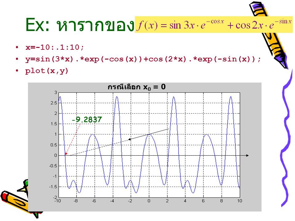
4 Ex: หารากของ x=-10:.1:10; y=sin(3*x).*exp(-cos(x))+cos(2*x).*exp(-sin(x)); plot(x,y)

5 เราจะหาคำตอบในช่วง [0, 2]
x =

6 MATLAB: Bisection Mtd. function [x]=example91a(es)
% Calculate using Bisection Method between [0,2] ea = inf; xr = inf; it=0; xl=0; xu=2; while(ea > es) it = it+1; pxr=xr; fxl=sin(3*xl).*exp(-cos(xl))+cos(2*xl).*exp(-sin(xl)); fxu=sin(3*xu).*exp(-cos(xu))+cos(2*xu).*exp(-sin(xu)); xr=(xl+xu)/2; fxr=sin(3*xr).*exp(-cos(xr))+cos(2*xr).*exp(-sin(xr)); ea = abs((xr-pxr)/xr)*100; x=[it xl fxl xu fxu xr fxr ea] if(fxl*fxr > 0.0) xl=xr; elseif (fxl*fxr < 0.0) xu=xr; else ea=0.0; end

7 Bisection Results:>> example91a(0.01)
Iter xl fxl xu fxu xr fxr ea x = Inf x = x = x = x = x = x = x = x = x = x = x = x = x = x = ans = x = True error = %

8 Other Results: xt= 0.95774795776341 Es = 0.01% Es = Es = 0.001%
It = 15;xr= Ea= %, et = % Es = Es = 0.001% It = 18;xr= Ea= %, et = % Es = % It = 21;xr= Ea= %, et = % Es = % It = 28;xr= Ea= %, et = e-008%

9 MATLAB: False-Position
function [x]=example91b(es) % Calculate using False-Position Method between [0,2] ea = inf; xr = inf; it=0; xl=0; xu=2; while(ea > es) it = it+1; pxr=xr; fxl=sin(3*xl).*exp(-cos(xl))+cos(2*xl).*exp(-sin(xl)); fxu=sin(3*xu).*exp(-cos(xu))+cos(2*xu).*exp(-sin(xu)); % xr=(xl+xu)/2; xr=xu-((fxu*(xl-xu))/(fxl-fxu)); fxr=sin(3*xr).*exp(-cos(xr))+cos(2*xr).*exp(-sin(xr)); ea = abs((xr-pxr)/xr)*100; x=[it xl fxl xu fxu xr fxr ea] if(fxl*fxr > 0.0) xl=xr; elseif (fxl*fxr < 0.0) xu=xr; else ea=0.0; end

10 FP Results:>> example91b(0.01)
Iter xl fxl xu fxu xr fxr ea x = Inf x = x = x = x = x = x = ans = x = True error = %

11 Other Results: xt= 0.95774795776341 สีน้ำเงินได้จาก Bisection Method
สีเขียวได้จาก False-Position Method Es = 0.01% It = 15;xr= Ea= %, et = % It = 7;xr= Ea= %, et = % Es = Es = 0.001% It = 18;xr= Ea= %, et = % It = 8;xr= Ea= %, et = % Es = % It = 21;xr= Ea= %, et = % It = 9;xr= Ea= %, et = % Es = % It = 28;xr= Ea= %, et = e-008% It = 10;xr= Ea= %, et = e-008%

12 Newton-Ralphson Method

13 MATLAB Program: function [x]=example91c(es,x0)
% Calculate solution using Newton-Ralphson, x0=initial; it=0; xi=x0; ea=inf; while (ea > es) it = it+1; fxi=sin(3*xi)*exp(-cos(xi))+cos(2*xi)*exp(-sin(xi)); dfxi=exp(-cos(xi))*(sin(3*xi)*sin(xi)+3*cos(3*xi))... -exp(-sin(xi))*(cos(2*xi)*cos(xi)+2*sin(2*xi)); pxi=xi; xi=pxi-fxi/dfxi; ea=abs((xi-pxi)/xi)*100; x=[it pxi fxi dfxi xi ea] end

14 Result: ea=0.01, xo=? X0=0 โปรแกรมจะ Converge เข้าสู่จุดอื่นด้านซ้าย
ดูรูป ถ้า x0 = 0.5 หรือ 1.5 โปรแกรมจะ Converge เข้าจุดที่ต้องการอย่างรวดเร็วมาก เป็นไปได้ที่เราเลือกจุดที่โปรแกรมไม่ Converge เราอาจจะใช้ Bisection Method ก่อนเพื่อหาจุด x0 ที่ดี จากนั้นต่อด้วย Newton-Ralphson เพื่อให้ได้คำตอบอย่างรวดเร็ว

15 เราจะหาคำตอบในช่วง [0, 2]
X0=0 x = 2.1310 X0=2

16 Ex: หารากของ x=-10:.1:10; y=sin(3*x).*exp(-cos(x))+cos(2*x).*exp(-sin(x)); plot(x,y) กรณีเลือก x0 = 0

17 Result: x0=0.5, es = 0.01 Iter xi fxi dfxi xi ea x = x = x = x = x = x = True error = %

18 Result: x0=0.5, es = Iter xi fxi dfxi xi ea x = x = x = x = x = x = x = True error = %

19 Compare : xt =0.95774795776341 Es = 0.01% Es = Es = 0.001%
It = 15;xr= Ea= %, et = % It = 7;xr= Ea= %, et = % It = 4;xi= Ea= %, et = % Es = Es = 0.001% It = 18;xr= Ea= %, et = % It = 8;xr= Ea= %, et = % It = 5;xi= Ea= %, et < 1.0e-15 % Es = % It = 21;xr= Ea= %, et = % It = 9;xr= Ea= %, et = % Es = % It = 28;xr= Ea= %, et = e-008% It = 10;xr= Ea= %, et = e-008% เพียง 5 iteration วิธีของ Newton-Ralphson ให้ Error น้อยจน Double Precision วัดไม่ได้ แต่ข้อเสียคือจุด x0 จะต้องเลือกให้ดี

20 Chapter 9: System of Linear Eq.
จะ Limit อยู่ที่สมการ AX=B โดย A เป็น Square Matrix N สมการ N Unknown จะมีคำตอบที่ Unique คำตอบจะมีได้ต่อเมื่อ A ไม่เป็น Singular Determinant ไม่เท่ากับ 0 A หา Inverse ได้ และ X = A-1B ในกรณีที่ Determinant A ใกล้ศูนย์ แต่ไม่ใช่ศูนย์ คำตอบจะ Sensitive กับ Error การคำนวณเมื่อมีการปัดเศษจะต้องระวัง กรณีนี้ เราเรียกว่ามันเป็น ‘Ill-Conditioned System’

21 System of Linear Equations

22 Krammer’s Rule

23 Solution ของ AX=C A-1AX=A-1C X=A-1C
Inverse หาได้ยาก แม้จะใช้ Computer คำนวณ เพราะเป็น O(n4)

24 Solution by Elimination

25 Gauss Elimination ใน Elimination Step จาก AX=C เราพยายามทำให้ Matrix A อยู่ในรูป Upper Diagonal Matrix ด้วยขบวนการ Elimination คือการบวกและลบแต่ละแถวเข้าด้วยกัน และค่า C จะถูกบวกลบตามไปด้วย เมื่อ A เป็น Upper Diagonal แล้ว การแก้สมการสามารถทำได้ง่าย โดยเราหา xn ก่อนในแถวสุดท้ายของสมการ จากนั้นนำ xn ที่หาได้มาแทนค่า เพื่อหา xn-1 ในแถวรองสุดท้าย เนื่องจากเป็นการแทนค่าเพื่อหา Unknown ย้อนหลัง เราจึงเรียก Back-Substitution

26 Gauss Elimination จาก

27 Gauss Elimination

28 Gauss Elimination

29 Gauss Elimination

30 Gauss Elimination

31 Gauss Elimination

32 Back Substitution

33 Back Substitution

34 Gauss Elimination

35 Gauss Elimination

36 Gauss Elimination

37 Gauss Elimination

38 Gauss Elimination

39 Gauss Elimination Alg Elimination by Forward Substitution

40 Gauss Elimination Alg Back-Substitution

41 Gauss Elimination Alg Back-Substitution

42 Example 8.1

43 Example 8.1

44 Example 8.1 Back Substitution

45 ปัญหาของ Gauss Elimination

46 ปัญหาของ Gauss Elimination

47 ปัญหาของ Gauss Elimination

48 ปัญหาของ Gauss Elimination

49 Gauss-Jordan Method

50 Gauss-Jordan Method

51 Example 8.2

52 Example 8.2

53 Example 8.2

54 Example 8.2

55 Example 8.2

56 Example 8.2

57 การหา Matrix Inverse ด้วย GJ

58 การหา Matrix Inverse ด้วย GJ

59 การหา Matrix Inverse ด้วย GJ

60 การหา Matrix Inverse ด้วย GJ

61 การหา Matrix Inverse ด้วย GJ

62 Example 8.3

63 Example 8.3

64 Example 8.3 จำนวนการคำนวณจะใช้น้อยกว่าวิธีทาง Analytic Method มาก

65 Iterative Method and Gauss-Seidel

66 Gauss-Seidel

67 Gauss-Seidel

68 Gauss-Seidel

69 Gauss-Seidel

70 Gauss-Seidel

71 Gauss-Seidel: Ex 8.4

72 Gauss-Seidel: Ex 8.4

73 Gauss-Seidel: Ex 8.4

74 Gauss-Seidel: Ex 8.4

75 Gauss-Seidel: Ex 8.4

76 Gauss-Seidel: Ex 8.4

77 Gauss-Seidel: Ex 8.4

78 Jacobi Method

79 Convergence of Iterative Method

80 Break After Break LU Decomposition

81 LU Decomposition

82 LU Decomposition

83 LU Decomposition

84 LU Decomposition

85 LU Decomposition

86 LU Decomposition

87 LU Decomposition

88 LU Decomposition

89 LU Decomposition

90 LU Decomposition

91 Crout Decomposition

92 Crout Decomposition

93 Crout Decomposition

94 Crout Decomposition

95 Crout Decomposition

96 Crout Decomposition

97 Crout Decomposition

98 Example 8.6

99 Crout Decomposition

100 Crout Decomposition

101 Example 8.7

102 Example 8.7

103

104 Summary Chapter 8

105 Homework 9 Chapter 9 DOWNLOAD
คำนวณแนะนำให้เขียนโปรแกรม หรือใช้ MATLAB หรือใช้ Spreadsheet(Excel)

106 End of Chapter 9 Next Week Chapter 10
Numerical Differentiation and Integration