ดาวน์โหลดงานนำเสนอ
งานนำเสนอกำลังจะดาวน์โหลด โปรดรอ

1
INC341 State space representation & First-order System
Lecture 3

2
Review บทที่ 2 เราศึกษาการแปลง physical model ให้เป็นสมการทางคณิตศาสตร์ โดยจะเขียนความสัมพันธ์ของ input/output ให้อยู่ในรูปของ transfer function ใน frequency domain ได้

3
Analysis and design of FCS
Classical Control วิเคราะห์ระบบใน Frequency domain (Ch. 2) Modern Control วิเคราะห์ระบบใน Time domain (Ch. 3)
 Modern Control. วิเคราะห์ระบบใน. Time domain. (Ch. 3)")
4
Chapter 3

5
Advantage and disadvantage of classical approach
Pros: สามารถตรวจสอบ stability ของระบบ สามารถดูผลของ transient response Cons: ใช้ได้แต่เฉพาะ linear, time-invariant systems และระบบnon-linear ที่ทำการ linearization แล้วเท่านั้น ไม่สามารถวิเคราะห์ระบบที่เป็น nonlinear และระบบที่มี non-zero initial condition ได้

6
Modern approach เป็นขบวนการที่สามารถประยุกต์ใช้ได้กับการสร้าง, วิเคราะห์, และออกแบบระบบโดยทั่วไปได้ โดยไม่คำนึงว่าระบบจะเป็น linear, time-invariant หรือไม่ก็ตาม อีกทั้งยังสามารถกำหนด initial condition ให้กับระบบได้อีกด้วย

7
State space representation
Classical Input Output System H(s) U(s) Y(s) Modern Input Output u(t) y(t)
 U(s) Y(s) Modern. Input. Output. u(t) y(t)")
8
State space representation (cont.)
State equation Output equation called controllable canonical form

9
State space representation
2-Dimension

10
Easy 2-D example ต้องการเขียน differential equation ข้างล่างนี้ให้อยู่ในรูป state space form

11
Converting transfer function to state space
Step 1: เริ่มต้นจากการแปลง transfer function ให้อยู่ในรูป differential equation ก่อน

12
Converting transfer function to state space (cont.)
Step 2: กำหนด state vector ใน differential equation ซึ่งจำนวน state vector จะเท่ากับ order ของ differential equation (n)
")
13
Converting transfer function to state space (cont.)
Step 3: จัดรูปใหม่ โดยเขียนให้อยู่ในรูปของ matrix A, B, C, และ D

14
Example 3.4 Insert Figure 3.10 here!!! Q: เริ่มทำยังไงก่อนดี???

15
Example 3.4 (cont.)
")
16
Example 3.4 (cont.)
")
17
Converting from state space to transfer function
Take Laplace transform

18
Example 3.6 Q: what are A, B, C, D???
Q: หลังจากรู้ A, B, C, D แล้ว ต้องทำยังไงต่อ???

19
Example 3.6 (cont.)
")
20
General view for transformation
differential equation classical approach modern approach transfer function state space

21
Matlab command Polynomial to transfer function: tf
State space to transfer function: ss2tf Transfer function to state space: tf2ss Demo!!

22
Chapter 4

23
Overview หลังจากที่เราได้สมการทางคณิตศาสตร์ของระบบที่เราจะทำการศึกษาแล้ว ต่อมาเราจะวิเคราะห์ดูผลของระบบทั้งในช่วง transient และ steady state โดยเนื้อหาในบทนี้ จะครอบคลุมถึงการศึกษาผลของระบบในช่วง transient เท่านั้น เช่นว่า ถ้าเราใส่ step input ไปในระบบจะได้ผลตอบสนองอย่างไร

24
Order of transfer function
Transfer function จะอยูในรูปเศษส่วน Polynomial เช่น Note: order ของระบบก็คือ order ของ transfer function หลังจากที่ clear factor เรียบร้อยแล้ว (เท่ากับจำนวน poles ของระบบ) Q: ระบบต่อไปนี้มี order เป็นเท่าไร???
 Q: ระบบต่อไปนี้มี order เป็นเท่าไร")
25
Analysis and design tool
เครื่องมือที่จะใช้พิจารณาการวิเคราะห์และออกแบบระบบก็คือ poles & zeros ของ transfer function ซึ่ง poles, zeros นี้สามารถบอกได้ถึง ความมีเสถียรภาพ (stability) ของระบบ ความไวในการเข้าสู่เสถียรภาพ
 ของระบบ. ความไวในการเข้าสู่เสถียรภาพ.")
26
Poles and Zeros Poles คือค่า root ของตัวส่วน (denominator) ที่ทำให้ transfer function มีค่าเป็น infinity หรือกล่าวอีกในหนึ่งก็คือ ค่าของ s ที่ทำให้ตัวส่วน มีค่าเป็น 0 Zeros คือค่า root ของตัวเศษ (numerator) ที่ทำให้ transfer function มีค่าเป็น 0 หรือกล่าวอีกในหนึ่งก็คือ ค่าของ s ที่ทำให้ตัวเศษ มีค่าเป็น 0 เช่น Pole อยู่ที่ -5 Zero อยู่ที่ -2
 ที่ทำให้ transfer function มีค่าเป็น infinity หรือกล่าวอีกในหนึ่งก็คือ ค่าของ s ที่ทำให้ตัวส่วน มีค่าเป็น 0. Zeros คือค่า root ของตัวเศษ (numerator) ที่ทำให้ transfer. function มีค่าเป็น 0 หรือกล่าวอีกในหนึ่งก็คือ ค่าของ s ที่ทำให้ตัวเศษ. มีค่าเป็น 0. เช่น. Pole อยู่ที่ -5 Zero อยู่ที่ -2.")
27
Pole-Zero Plot jω s - plane -3+2j X O σ 2 -3-2j X
Plot of poles, zeroes on the s-plane Useful for system analysis

28
Unit step u(t) แปลง Laplace ได้ 1/s Pole-zero plot
 แปลง Laplace ได้ 1/s Pole-zero plot")
29
Poles จาก input จะให้ forced response
Poles จาก transfer function จะให้ natural response Amplitude เป็นผลจากทั้ง Poles และ Zeros

30
Type of Systems First-order Systems Second-order Systems
Higher-order Systems

31
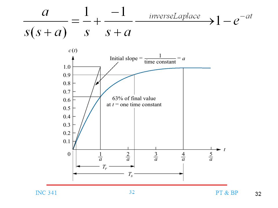
First-order Systems

33
Time constant = 1/a = ระยะเวลาที่ response ขึ้นถึง 63%
ของค่า final value Rise Time (Tr) = ระยะเวลาที่ใช้เพื่อให้ response ขึ้นจาก 0.1 ไป 0.9 ของค่า final value Settling Time (Ts) = ระยะเวลาที่ใช้เพื่อให้ response ขึ้นจาก 0 ไป 0.98 ของค่า final value
 = ระยะเวลาที่ใช้เพื่อให้ response ขึ้นจาก 0.1. ไป 0.9 ของค่า final value. Settling Time (Ts) = ระยะเวลาที่ใช้เพื่อให้ response ขึ้นจาก 0. ไป 0.98 ของค่า final value.")
34
Matlab commands Poles of transfer function: pole
Zeros of transfer function: zero Step input response: step

35
Type of Systems First-order Systems Second-order Systems
Higher-order Systems เน้น

36
1st order review Time constant = 1/a
Settling Time (Ts) = 4 เท่าของ time constant
 = 4 เท่าของ time constant.")
งานนำเสนอที่คล้ายกัน


 การแปลงฟูริเยร์แบบเร็ว>")


 98.08% 100.02% จังหวัด.>")


